ABSTRACT

The problem facing by physicians is the fact that for most drugs there is a minimum concentration below which the drug is ineffective, and a maximum concentration above which the drug is dangerous. Thus, this paper discusses the effective medicine dosage and its concentration in bloodstream of a patient. For analysis of dose concentration and mathematical modelling of minimum and maximum concentration of a drug administered intravenously, the EDM (Exponential Decay Model) and GSF (Geometric Series and its Formula) are the powerful mathematical tools. In the present research study, these two mathematical tools were used to predict the dose concentration of a drug in bloodstream of a patient.

1. INTRODUCTION

One of the physician’s responsibilities is to give medicine dosage for a patient in an effective manner. In this research study, the effective medicine dosage and its concentration in bloodstream of a patient are discussed in detail using two mathematical techniques: one is EDM (Exponential Decay Model) and other one is GSF (Geometric Series and its Formula). The EDM is very useful technique for simulating the dose concentration of a drug over time and GSF plays a vital role in modelling the minimum and maximum concentration of a drug administered intravenously.

2. EXPONENTIAL GROWTH AND DECAY

Exponential growth and decay are rates; that is, they represent the change in some quantity over time.

2.1. Exponential Growth Model

A quantity say is said to be subject to exponential growth, , if the quantity increases at a rate proportional to its value over time. Symbolically, this can be expressed as follows:

 

That is, , which is a differential equation.

where 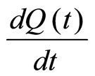is the rate of change of quantity over time, is the value of the quantity at time, and is a positive number called the growth constant.

Now, we can find solution for the differential equation

By rearranging this equation, we get

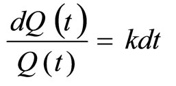
and then, by integrating this equation, we hav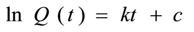e where is the constant of the integration.

By simplifying this equation, we get

.

We can obtain 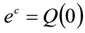by evaluating the equation 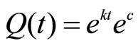at and is the initial value of the quantity that is denoted by for our convenience.

Therefore, 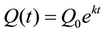, which is called the Exponential Growth Model.

2.2. Exponential Decay Model (EDM)

A quantity is said to be subject to exponential decay, , if the quantity decreases at a rate proportional to its value over time. Symbolically, this can be expressed as follows:

 

That is, 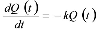where the negative sign ‘–‘ means the decrease in the quantity over time.

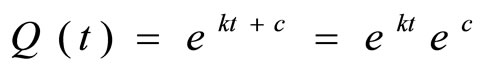
By solving this differential equation, we obtain 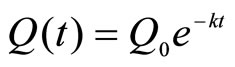, which is called the Exponential Decay Model (EDM).

Remarks: In general, and are exponential functions.

2.3. Geometric Series and its Formula (GSF)

Traditionally, geometric series played a key role in the early development of calculus, but today, the geometric series have many key applications in medicine, biochemistry, informatics, etc.

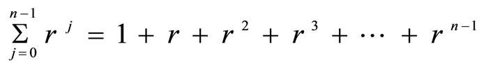
Usually, a geometric series is the sum of the terms of the geometric sequence:

.

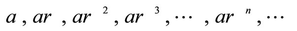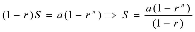
Now, the sum of the geometric sequence of n terms is denoted by

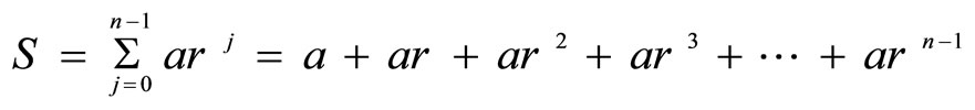
where denotes the sum, the first term, the ratio, and the number of terms.

.

When,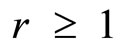

().

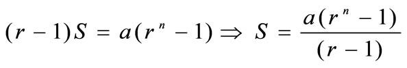and when or,

where 

.

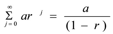
In the geometric series, the first term shows a = 1.

Thus, 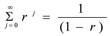when

3. EDM AND GSF IN EFFECTIVE MEDICINE DOSAGE

In this section, we discuss about the effective medicine dosage using Exponential Decay Model (EDM) and Geometric Series and its Formulae (GSF). Let us consider a patient is given the same dose of a medicine at equally spaced time intervals. The dose concentration in the bloodstream decreases as the drug is broken down by the body. However, it does not disappear completely before the next dose is given. Let us understand the exponential decay model for the concentration of a drug in a patient’s bloodstream. It is assumed that the drug is administered intravenously and that the concentration of the drug in the bloodstream jumps almost immediately to its highest level, i.e. the concentration of the drug decays exponentially.

Now, we use the function to represent a dose concentration at time t and to represent the concentration just after the dose is administered intravenously. Then the exponential decay model is formulated by

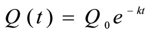
where k is the decay constant or a property of the particular drug being used.

Now, let us consider that be the first dose concentration at time t and thatthe concentration at time t = 0 just after the first dose is administered intravenously. Suppose that at t = c, a second dose of the drug is given to the patient. The concentration of the drug in the bloodstream jumps almost immediately to its highest level and then the concentration is diffused so rapidly throughout the bloodstream over time (Figure 1).

The expression 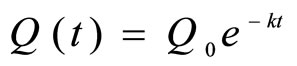is valid as long as only a single dose is given [1]. However, suppose that, at t = c, a second dose is given and that the amount of thedrug administered is the same as the first dose. Ac-

cording to the exponential decay model, the concentration will jump immediately by an amount equal to when the second dose is given. However, when the second dose is given, there is still some of the drug in the bloodstream remaining from the first dose. This means that to compute the concentration just after the second dose, we have to add the value to the concentration remaining from the first dose (Figure 1). During the time between the second and third doses, the concentration decays exponentially from this value. To find the concentration after the third dose, the same process must be repeated.

At t = c, the dose concentration is calculated as just before the second dose is administered intravenously.

Here,.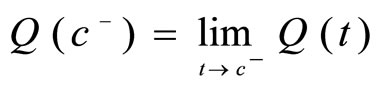

When the second dose is administered intravenously, the concentration jumps by an increment, i.e. the concentration just after the second dose given is

.

Note that denotes ‘just before the new dose is administered’ and 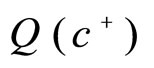denotes ‘just after the new dose is administered’.

The concentration then decays from this value according to the exponential decay rule [2], but with a slight twist. The twist is that the initial concentration is at t = c, instead of t = 0. One way to handle this is to write the exponential term as 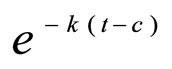so that at t = c, the exponent is 0. If we do this, then we can write the concentration as a function of time as

This function is only valid after the second dose is administered and before the third dose is given. That is, for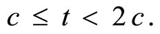

Now, suppose that a third dose of the drug is given at t = 2c. The concentration just before the third dose is given would be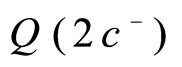, which is

i.e.,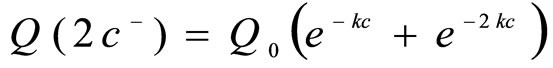

When the third dose is given, the concentration would jump again by and the concentration just after the third dose would be

Now, suppose that a forth dose of the drug is given at t = 3c. The concentration just before the forth dose is given would be, which is

When the third dose is given, the concentration would jump again by and the concentration just after the third dose would be

Let us consider the process is continued up to n-th dosei.e.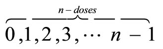

The concentration just before the n-th dose of the drug would be

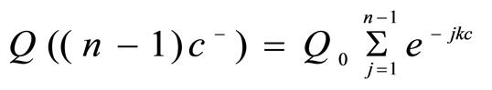(1)

The concentration just after the n-th dose of the drug would be

(2)

Let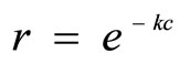

Note that, since k and c are both positive constants.

From the geometric series (1) and (2), we formulate as

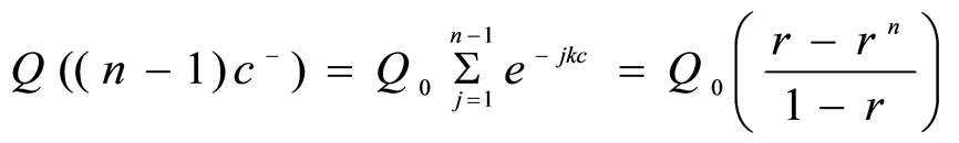(3)

and

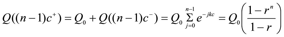(4)

The Eqs.3 and 4 are formulae for the partial sum of a geometric series.

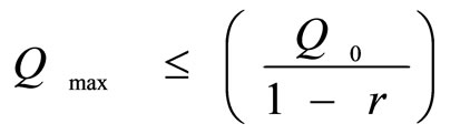
Suppose a treatment for a patient is continued indefinitely. Then the Eq.4 becomes

.

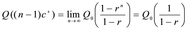
Now, we conclude from the results that the minimum concentration is the concentration just before the second dose is giveni.e. 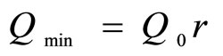and that the maximum concentration is the concentration just after the last dose is given, i.e.

4. DISCUSSION

For example, a patient is injected a particular drug. Just after the drug is injected, the concentration is 1.5 mg/ml (milligrams per milliliter). After four hours the concentration has dropped to 0.25 mg/ml.

Here, at t = 4 and 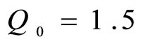at t = 0. So,.

To find k, Maple commands were used [8].

Result: k = 0.4479398673.

A problem facing physicians is the fact that for most drugs, there is a concentration, below which the drug is ineffective and a concentration, above which the drug is dangerous. Thus, the concentration must satisfy the condition: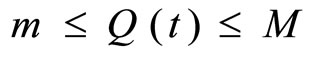. For example, suppose that for the drug in the experiment [8] the maximum safe concentration is 5 mg/ml, or M = 5, and the minimum effective concentration is 0.6 mg/ml, or m = 0.6. Then the initial dose must not produce a concentration greater than 5 mg/ml.

5. CONCLUSIONS

In the research study, the EDM (Exponential Decay Model) and GSF (Geometric Series and its Formula) discuss in detail for effective medicine dosage. Especially the two techniques have been used for analysis of dose concentration in bloodstream of a patient and modelling of minimum and maximum concentration of a drug administered intravenously.

REFERENCES