Modern Economy
Vol. 3 No. 8 (2012) , Article ID: 26288 , 9 pages DOI:10.4236/me.2012.38120
The Effect of Federal Government Size on Long-Term Economic Growth in the United States, 1791-2009
Department of Economics, University of Nevada, Reno, USA
Email: guerrero@unr.edu, eparker@unr.edu
Received September 4, 2012; revised October 18, 2012; accepted October 28, 2012
Keywords: Long-Term Economic Growth; Federal Government Size; Wagner’s Law; United States; Cointegration; Granger Causality; Vector Autoregression; Vector Error Correction Model
ABSTRACT
We consider whether there is statistical evidence for a causal relationship between federal government expenditures and growth in real GDP in the United States, using available data going back to 1791. After studying the time-series properties of these variables for stationarity and cointegration, we investigate Granger causality in detail in the context of a Vector Error Correction Model. While we find causal evidence that faster GDP growth leads to faster growth in government spending, we find no evidence supporting the common assertion that a larger government sector leads to slower economic growth.
1. Introduction
Is a larger government bad for growth? Much of the current U.S. debate over economic stimulus versus debt reduction assumes that public spending dampens economic growth in the long run, and thus tax cuts are a more effective policy. However, both the theoretical effects of government size and the empirical record are much more mixed than the US political dialogue asserts.
In theory, government expenditures can have both short-run fiscal effects on aggregate demand, at least in an economy with excess capacity, as well as at least seven separate long-run effects, including the provision of pure and quasi-public goods, the distortionary effect of taxes on resource allocation, and the comparative inefficiency of government control over resources and production, relative to the private sector it replaces [1]. As a result of these positive and negative effects, Barro [2] has made a persuasive case that the aggregate relationship between the size of government and economic growth may be shaped like an inverted-U, with low growth resulting from both too little and too much government. The marginal long-run effect of government size would thus be zero for an economy at the optimum.
Empirical results are also mixed, especially with international comparisons. Landau [3,4] found a negative effect of government consumption on growth, while Ram [5] found a positive effect. Lee and Lin [6] found a negative effect of government that disappeared once demographic factors were taken into account. In his surveySlemrod [7] argues that the aggregate effect of government involvement is negligible, though some types of taxes affect some behaviors significantly. Engen and Skinner [8] focus on the effect of taxes, and they find mildly negative effects for some taxes and positive effects for others, but like much of the rest of the literature, the effects of larger government are contradictory, ambiguous, and in the aggregate rather minimal.
Plümper and Martin [9] found a negative effect of government on growth primarily in non-democratic countries, a result generally consistent with the findings of Guseh [10] and Scully [11]. Poot [1] cited 41 studies, with seven finding a positive effect, twelve finding a negative effect, and 23 inconclusive. The bivariate causal relationship between government size and economic growth is complicated by the potential for reverse causation, since GDP growth can also lead to increased government spending, an effect that is frequently referred to, in a broad sense, as Wagner’s law [12]. As Baumol and Bowen [13] first noted for the example of orchestras, many labor-intensive services have inherently lower rates of productivity improvement, while wages are driven by productivity improvements elsewhere.
Wagner’s law has also been interpreted to imply an income elasticity for government expenditures greater than one, although Peacock and Scott [14] argue that this relationship is usually specified incorrectly. As with the previous causal relationship, there is also a substantial literature testing whether economic growth leads to a larger government. Recent examples include Jackson, Fehti and Fehti [15], Demirbas [16], Islam [17], and Halicioglu [18].
A common methodological pitfall in the literature that tries to uncover the causal links between government size and long-term economic growth is that these studies regularly conduct Granger causality tests outside the cointegration framework, though Jones and Joulfain [19], Ghali [20] and Islam [17] are among the exceptions. As is now well-known, this problem may render many of their conclusions invalid [21]. Furthermore, the papers that do place their Granger causality analyses within the cointegration framework do not tend to implement a Vector Error Correction (VEC) model, which is the natural follow up in the case in which the variables are cointegrated, given that the definitive test of causality lies with the error correction term [21,22].
In this paper, we complement the previous contributions of Jones and Joulfain [19] and Islam [17], both of which address causation issues within the cointegration framework. We focus on federal government outlays, not government revenues—which are more clearly driven in the short-run by changes in GDP—or the financing through debt. In the latter case, the fiscal and time-series properties were thoroughly explored by Kremers [23], using data from 1920-1985. While Jones and Joulfain [19] study the relationship between federal government receipts and outlays in the period up to the American civil war and Islam [17] tests the validity of Wagner’s law during the period 1929-1996, we have the advantage of using a long dataset covering the period 1791-2009. Our longer dataset allows us to test different causation hypothesis more precisely and also study the stability of results over different periods of time, a task that our predecessors could not tackle, given the limitations imposed by the available data.
We begin in section two with a brief description of government size and economic growth over the longterm for the case of the US, using data going back to 1791. In section three, we study the time series properties of the data, testing for stationarity and cointegration. In the fourth section we exploit the results from cointegration analysis and implement a VEC model that sheds clear light on the issue of causation. We conclude with a brief summary and suggestions for further research.
2. The Size of the US Government
There are many ways to measure the size and scope of government intervention, but the most common metric is the relative amount of government expenditures, including both government purchases and transfers. In the US, federal government expenditures as a share of GDP remained low prior to the Great Depression, with exception to wartime. This ratio then dramatically increased during the Roosevelt Administration, but in the postwar period it generally ranged below 25%. State and local expenditures, meanwhile, actually fell during the Roosevelt Administration.
From the Truman Administration through the Reagan Administration, government spending continued to rise, to an average of 23% of GDP for federal spending in the first half of the 1980s (and an average of almost 11% of GDP for state and local expenditures). By the first half of the 1990s, government expenditures in the United States totaled a third of GDP.
How did this secular increase in government size affect growth on the margin in the United States? Gwartney, Lawson, and Holcombe [24] argued that the size of government in the first half of the 1960s was close to the optimal level, and estimated that US incomes would have been 20% in 1996 had government stayed the same relative size, but they chose to make their case using the period 1960-65 as their growth baseline, a half-decade with the highest growth rates in postwar American history.
To more carefully analyze the effect of government spending on growth, we compile annual GDP data for the United States, both current and real, using the Historical Statistics of the United States [25] and the US Department of Commerce’s Bureau of Economic Analysis [26]. Annual federal outlays are also available from the first source above, with more recent data from the Office of Management and Budget.
For several reasons, including differences between the calendar year and the fiscal year, these data on annual federal outlays do not precisely match the BEA data on current federal expenditures, which are not available before 1929. To approximate federal purchases, these spending data are adjusted by subtracting out expenditures on veterans’ pensions, Social Security, and Medicare, though again the resulting data do not exactly match the BEA data on federal purchases, which are not available before 1929.
These data are shown in Figure 1, as a percentage of the 1800-2000 trended real GDP. It is clear that with the exception of wartime (e.g., the Civil War of 1861-65, the First World War and the Second World War), the growth in federal outlays occurred primarily between 1930 and 1950. It also appears from this figure that US GDP growth hit its peak during the twenty years from 1890 to 1910, although as Table 1 shows this was primarily the result of immigration and population growth. The standard deviation of growth was generally smaller after 1950, suggesting that the growth of government was not only correlated with faster growth, but also correlated with more economic stability. While federal government expenditures were a much higher share of GDP after the Roosevelt Administration than before, this ratio also became much more stable.
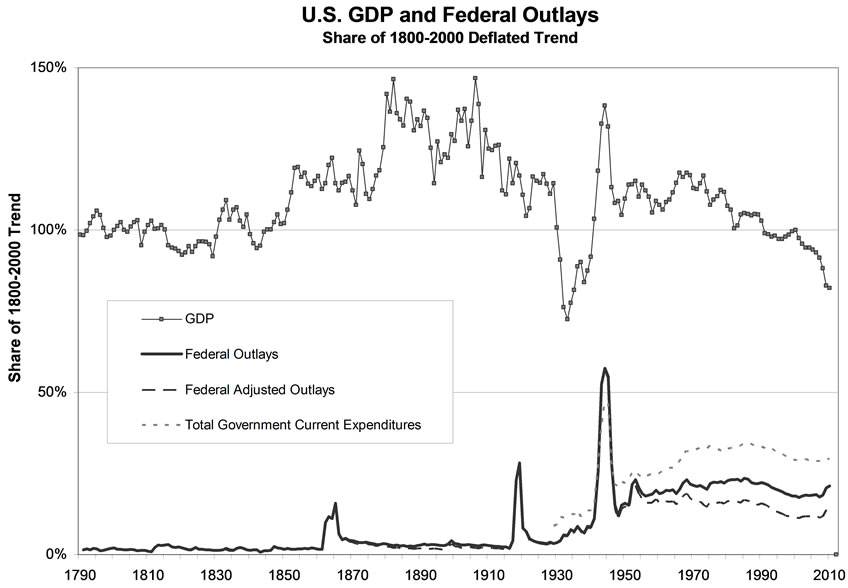
Figure 1. US GDP and federal outlays, adjusted for trend.
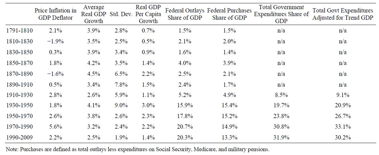
Table 1. US GDP and federal outlays, 1791-2009.
Figure 1 also shows the BEA data for overall current expenditures by all governments in the US, including state and local spending. Unfortunately, these data are not available before 1929 in consistent form, so we will save the analysis of the effect of state and local government spending for another paper. Like Jones and Joulfain [19], who investigate the relationship between expenditures and revenues prior to the Civil War, we focus on the federal budget and exclude state and local government expenditures from our analysis because of data availability. This figure suggests that the current rise in federal expenditures during the present recession appears to be primarily offsetting the decline in state and local government spending, and the increased ratio is primarily a result of declining GDP growth, not faster growth in government spending.
Is the marginal effect of government bad for economic growth in the US? The United States had the smallest total government expenditure share of all the OECD countries in the mid-1990s, and also the smallest growth in government’s share during the postwar period. If any developed market economy is on the lower, upwardsloping portion of the Barro curve, it seems likely that it should be the United States.
Islam [17] investigated the relationship between total government expenditures and growth in order to test for Wagner’s law, using U.S. data from the U.S. Department of Commerce spanning the period 1929-1996, and found a long-term equilibrium relationship between economic growth and the share of government expenditures, with causality that supported Wagner’s law but not the reverse. Like Islam, we estimate whether or not such a cointegrating relationship exists for the US, though we consider a much longer time-series and we investigate both causality issues and the dynamic relationship in more detail.
Others have used similar methods to investigate this question for other countries, or in other cases. One of the earlier examples is that of Conte and Darrat [27], who use Granger causality tests to reject the hypothesis that public sector expansion in postwar OECD economies negatively influenced real GDP growth rates. Ghali [20] used a multivariate cointegration approach with several variables, including GDP and government spending among others, for a sample of OECD countries, while Jones and Joulfain [19] used cointegration tests and error correction models to find evidence of short-term and long-term causality relationships in the United States between federal revenues and expenditures.
3. Stationarity and Cointegration
We begin by defining annual real GDP as Y, and real federal government expenditures as G, the sum of both government purchases (GP) and government transfers (GT). Transfers are assumed to include only three components that could be easily separated out for the 1791- 2009 period, namely expenditures for Social Security, Medicare, and military pensions. As a result, government purchases are overstated by transfers to state and local governments that are in turn transferred to the public. The ratio of federal government expenditures to GDP (G/Y) is defined as g, where g = gp + gt. The variables to be used in the analysis are lnY, lng, lngp, and lngt. Summary statistics are shown in Table 2.
In this analysis, we also consider the full sample from 1791-2009 as well as a truncated sample from 1791-1945, which excludes the postwar period in which the role of the US federal government fundamentally changed, and in which transfers became a significant portion of overall expenditures. By using the longer samples for comparison, we are better able to take advantage of the timeseries properties.
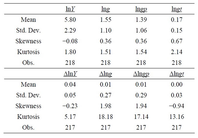
Table 2. Summary statistics.
Stationarity and cointegration are the first steps of analysis, because if the variables turn out to be non-stationary in their levels and are cointegrated, then the Vector Error Correction (VEC) model is the appropriate analytical tool to use. This model improves the econometric fit by tying the short-run dynamics to the long-run relationship between both variables. On the other hand, if the variables are not cointegrated, then VEC restrictions would not be appropriate.
We tested for the significance of a deterministic linear trend and found it to be significant in all cases, so all the tests include a deterministic linear trend. The PhillipsPerron tests results for unit roots in the variables’ levels are shown in Table 3.
For those two cases, it is useful to reverse the null hypothesis and test the null of stationarity instead with the Kwiatkowski-Phillips-Schmidt-Shin test [28]. This strategy of reversing the null increases the power of the tests, and turns out to be successful. The null hypothesis of stationarity yields LM statistics of 0.23 and 0.21 respectively, statistics that can be rejected at all levels of significance. We thus conclude that real GDP and the three ratios of federal government expenditures over GDP are all non-stationary in their log-levels, and this raises the question about whether or not they are cointegrated.
Table 4 shows the results of these Johansen tests. The log-level of real GDP displays a long-term equilibrium relationship with the log-levels of all three government spending ratios. Furthermore, at the 1% level, the trace test statistic indicates the existence of only one cointegration relationship.
These tests provide a uniform message for the truncated sample, namely that all variables are non-stationary in their levels. For the full sample, the message is somewhat less clear in regards to two variables, lng and lngp. In those two cases the null hypothesis of a unit root (i.e., non-stationarity) can only be rejected at the 1% level, but not at the 5% level.
If the variables are cointegrated, causality tests conducted outside the cointegration analysis framework may lead to incorrect causal inferences, since the error correction term is omitted in the specifications used to test for

Table 3. Phillips-Perron unit root tests.
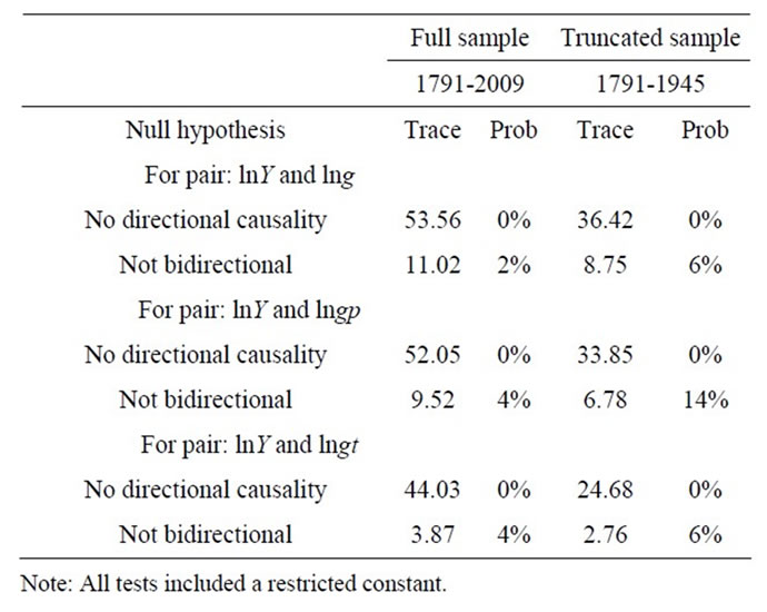
Table 4. Johansen pairwise cointegration tests.
Granger causality [21]. Here we follow Johansen’s onestep procedure to conduct cointegration analysis and Granger causality tests within the VEC framework. Engle and Granger [29] have also shown that if two variables are cointegrated, then a VEC model linking these variables must exist. Furthermore, the VEC model representation of the bivariate system of cointegrated variables sheds light on the direction of causation between those variables.
4. A Vector Error Correction Model
Engle and Granger [29] have shown that if two variables are cointegrated, then a VEC model exists to link these variables, and this representation of the bivariate system illuminates the direction of causation between those variables [21]. This VEC model is formulated in first differences as follows:
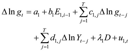
where the error correction terms are given by Ei,t-1, a matrix of dummy variables is given by D, ci and di are the autoregressive parameters, and T is the number of lags to be included. Nonzero values of ai means that a deterministic time trend exists in the data, while the λi terms yield changes in that trend associated with dummy variables that correspond to the US Civil War (1862-65), World War I (1916-18), World War II (1942-45), and the Postwar period (1946-2009). We also tried a post-1965 dummy variable to proxy for the creation of Medicare and the implied expansion of the welfare state, but found it to be statistically insignificant.
The VEC model specified allows for bivariate Grangercausality between the lnY and lng variables, so long as the corresponding error correction term carries a statistically significant coefficient, even if the estimated dj coefficients are not jointly statistically significant [21]. If these variables are cointegrated, then the error correction terms are stationary I(0) processes. Conversely, if the residuals from the static regressions are I(0), then the variables involved are cointegrated [29].
Residuals need to be orthogonalized in order to isolate the influence of each variable’s impact on the other variable. One method to do this is to use a structural vector auto-regression model, which requires prior knowledge to create the proper identifying restrictions. Because we take no stand on prior knowledge of the identifying restrictions, we use an alternative Cholesky factorization method that forces the system of equations to be a lower triangular matrix with strictly positive diagonal entries.
A potential problem with the Cholesky factorization method is that ordering the variables in different ways can produce different results if the residuals are correlated, and this could alter the conclusions of the test. This problem is minimized by using a model in which the ordering of the variables is based on their ex ante exogeneity, so that exogenous variables with the most predictive power are placed first, while endogenous variables are placed last. The results of pre-testing the variables for their degree of exogeneity are summarized in Table 5, and they clearly indicate that lnY is more ex ante exogenous than either lng or lngp, though results were inconclusive for transfers. To ensure the robustness of our results, all tests also use reverse ordering, which don’t substantially change our conclusions.

Table 5. Pre-testing for exogeneity, granger causality.
We estimate VEC models for the interaction between real GDP, measured as lnY, and the ratio of federal government expenditures to GDP, measured as lng, entered in that order. We also estimate each model for a truncated sample as well as the full sample, to determine whether the growth of federal government size, especially in transfer payments, in the postwar period significantly affects the results.
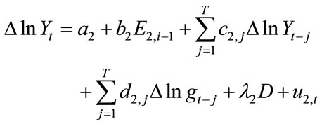
In Figure 2, we show the impulse-response diagrams derived from these VEC model estimations. These diagrams show the accumulated responses of lnY to onestandard-deviation Cholesky innovations in both lnY and lng, as well as the reverse exercise in which the responses of lng to shocks in lnY and lng.
As the upper right diagram in Figure 2(a) shows, we can reject the hypothesis that changes in government spending reduce real GDP. Indeed, the accumulated im-
 (a)
(a) (b)
(b)
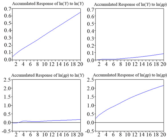
Figure 2. Impulse-response for GDP and expenditures. (a) Full sample: 1791-2009; (b) Truncated sample: 1791-1945.
pact of an orthogonalized shock to government spending is positive during the 20-year window of the experiment.
The lower left diagram shows some evidence in support of Wagner’s law, in that a positive Cholesky shock to real GDP leads to a consistent but modest increase in government spending between periods 3 and 20. Finally, the response of lnY to its own orthogonalized shocks shows a well-known linearly-persistent pattern with a slope smaller than unity, and the response of lng to its own orthogonalized shocks displays a pattern of increasing concavity in which the responses are persistent but diminishing.
For the truncated sample in Figure 2(b), the pattern is similar. The accumulated response of lnY to lng is significantly positive when accumulated over 20 years, and still positive but very modest in a period of 6 years or less. The accumulated response of lng to lnY is also similar but larger in proportion, most likely because g is smaller on average in the truncated sample.
Table 6 shows that the residuals from the VEC(4) model used to derive the impulse-response results, for both full and truncated samples, for g, gp, and gt. These residuals are mostly free of autocorrelation; the only lag for which the hypothesis could not be rejected is lag 2. As Johansen and Juselius (1990) have shown, the fact that the residuals are uncorrelated is critical for cointegration analysis (though deviations of the residuals from normality are not).
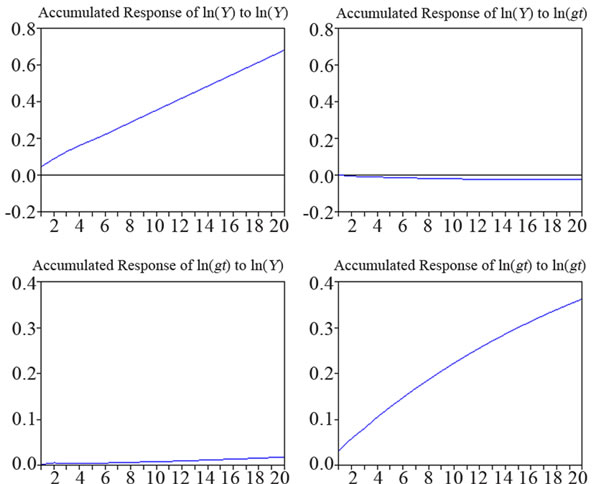
In Figure 3, we show the impulse-response diagrams for federal government purchases, i.e., outlays less expenditures on Social Security, Medicare, and military pensions. As this impulse-response diagram shows, our results are robust to the definition of federal government spending used, and the truncated sample does not yield substantially different results. The middle columns of Table 6 again show that autocorrelation only shows up in the second lag.
The impulse-response exercises just conducted clearly illustrated the relative importance of the quantitative effects involved when each variable is allowed to act as an exogenous shock: changes in federal government outlays have modest effects on real GDP, especially at short horizons, but increases in real GDP display strong positive effects on federal government outlays even at short horizons. This is not a new result, and it has been found before by other papers that conducted causality tests within the appropriate cointegration framework, such as Islam [17], which uses a different dataset from the Department of Commerce, a shorter sample (1929-1997), and no dummy variables.
However, if we consider transfers only, i.e., expenditures on Social Security, Medicare, and military pensions, we get different results. Figure 4 reports these impulseresponses results.

Table 6. VEC residual serial correlation LM tests.
 (a)
(a)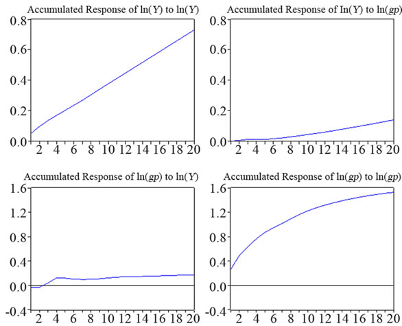 (b)
(b)
Figure 3. Impulse-response for GDP and purchases. (a) Full sample: 1791-2009; (b) Truncated sample: 1791-1945.
 (a)
(a)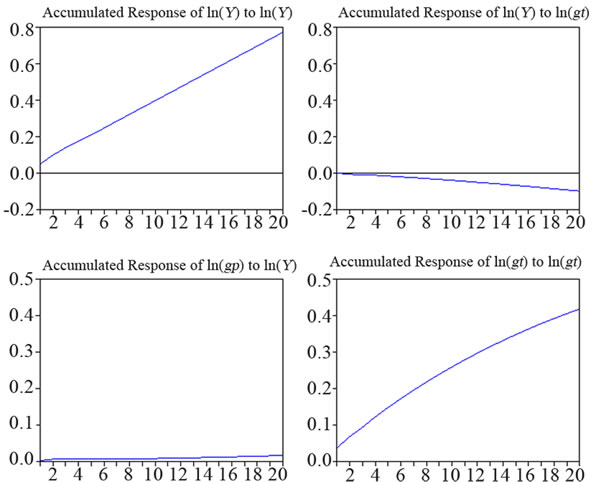 (b)
(b)
Figure 4. Impulse-response for GDP and transfers. (a) Full sample: 1791-2009; (b) Truncated sample: 1791-1945.
In both the full and truncated samples, these impulseresponse diagrams suggest that the impact of transfers on real GDP is negative, though in the first sample it is insignificantly small, while the impact of real GDP on transfers is essentially zero, showing no general trend supporting Wagner’s law. The slightly larger negative effect of gt on Y in the truncated sample was during a period in which transfers were a minor share of government spending, before the welfare state was fully developed. We also do not find evidence of autocorrelation in the residuals.
We then estimate this VEC model for the smaller postwar sample, though the number of observations is too limited for high confidence and we do not report the results. The resulting impulse-response diagrams indicated that an increase in government transfers had a significantly positive long-run effect on real GDP, and viceversa. This result, which should be taken with a grain of salt, suggests that transfers may not result primarily from rent-seeking activities, but might instead reduce otherwise uninsurable risks. Of course, these impulse-response diagrams do not necessarily infer causality.
The causality results implied by both Granger tests conducted within the VEC model and the error-correction terms contained in the simultaneous estimation of equations are generally unambiguous: causality runs from lnY to lng in all cases and not generally the other way round, confirming the results obtained at the pretesting stage.
There is thus no evidence whatsoever that a bigger government reduces economic growth, though there is compelling support for Wagner’s law that rising income leads to a rising share of government spending, for both total federal expenditures and purchases, but not for transfer payments.
5. Conclusions
A number of studies over the past two decades have considered whether a larger government is good or bad for growth. In this paper we complement our predecessors’ findings by using a longer dataset comprising annual data for federal government expenditures and real per-capita GDP for the United States going back to 1791. Our longer dataset permits a careful study of the time-series properties of these variables for stationarity, cointegration, and Granger causality, a series of steps some studies have begun but not completed, and some others could not conduct in full because of short samples and other data limitations.
After a careful study of the issue of causation within the cointegration framework, we find support for the argument that faster growth in the United States may lead to a larger government in the long run, but we do not find significant evidence supporting the hypothesis that the relative size of federal government expenditures affects growth, either up or down. This suggests the size of the federal government in the United States is, in fact, near the peak of the Barro curve.
Our results confirm the validity of many of the quailtative results reported by Islam [17], even though our sample size was much longer, and our investigation and our focus was on uncovering the relationship running from government size to economic growth rather than the reverse. It remains to be seen, however, whether these results can be generalized to other countries. Relative to other countries at similar levels of development, the US is somewhat of an outlier in that the relative size and role of government is less and the growth in government’s size has been much less, as well.
In closing, we note an important limitation of our study, in that we do not have the data necessary to either consider the effects of state and local government, or to control for other growth determinants in these regressions. Thus, much work remains to improve our understanding of the causal relationship between the share of government spending and long-term economic growth.
REFERENCES
- J. Poot, “A Synthesis of Empirical Research on the Impact of Government on Long-Run Growth,” Growth and Change, Vol. 31, No. 4, 2000, pp. 516-546. doi:10.1111/0017-4815.00143
- R. J. Barro, “Government Spending in a Simple Model of Endogenous Growth,” Journal of Political Economy, Vol. 95, No. 5, 1990, pp. S103-S125. doi:10.1086/261726
- D. Landau, “Government Expenditure and Economic Growth: A Cross-Country Study,” Southern Economic Journal, Vol. 49, No. 3, 1983, pp. 783-792. doi:10.2307/1058716
- D. Landau, “Government and Economic Growth in the less Developed Countries: An Empirical Study for 1960- 80,” Economic Development and Cultural Change, Vol. 35, No. 1, 1986, pp. 35-75. doi:10.1086/451572
- R. Ram, “Government Size and Economic Growth: A New Framework and Some Evidence from Cross-Section and Time-Series Data,” American Economic Review, Vol. 76, No. 1, 1986, pp. 191-203.
- B. S. Lee and S. Lin, “Government Size, Demographic Changes, and Economic Growth,” International Economic Journal, Vol. 8, No. 1, 1994, pp. 91-108.
- J. Slemrod, “What Do Cross-Country Studies Teach about Government Involvement, Prosperity, and Economic Growth?” Brookings Papers on Economic Activity, Vol. 1995, No. 2, 1995, pp. 373-431.
- E. M. Engen and J. Skinner, “Taxation and Economic Growth,” National Tax Journal, Vol. 49, No. 4, 1996, pp. 617-642.
- T. Plümper and C. W. Martin, “Democracy, Government Spending, and Economic Growth: A Political-Economic Explanation of the Barro-Effect,” Public Choice, Vol. 117, No. 1-2, 2003, pp. 27-50. doi:10.1023/A:1026112530744
- J. S. Guseh, “Government Size and Economic Growth in Developing Countries: A Political-Economy Framework,” Journal of Macroeconomics, Vol. 19, No. 1, 1997, pp. 175- 192. doi:10.1016/S0164-0704(97)00010-4
- G. W. Scully, “Economic Freedom, Government Policy and the Trade-Off between Equity and Economic Growth,” Public Choice, Vol. 113, No. 1-2, 2002, pp. 77-96. doi:10.1023/A:1020308831424
- A. Wagner, “Grundlegung der Politischen Ökonomie,” 3rd Edition, Winter’sche Verlagshandlung, Leipzig, 1892.
- W. J. Baumol and W. G. Bowen, “On the Performing Arts: The Anatomy of Their Economic Problems,” American Economic Review, Vol. 55, No. 1-2, 1965, pp. 495- 502.
- A. Peacock and A. Scott, “The Curious Attraction of Wagner’s Law,” Public Choice, Vol. 102, No. 1-2, 2000, pp. 1-17. doi:10.1023/A:1005032817804
- P. M. Jackson, M. D. Fehti and S. Fehti, “Cointegration, Causality and Wagner’s Law: A Test for Northern Cyprus, 1977-1996,” 2nd International Congress on Cyprus Studies, Gazimağusa, 24-27 November, 1998, pp. 1-24.
- S. Demirbas, “Cointegration Analysis-Causality Testing and Wagner’s Law: The Case of Turkey, 1950-90,” European Public Choice Society, Lisbon, 1999.
- A.M. Islam, “Wagner’s Law Revisited: Cointegration and Exogeneity Tests for the USA,” Applied Economics Letters, Vol. 8, No. 8, 2001, pp. 509-515. doi:10.1080/13504850010018743
- F. Halicioglu, “Testing Wagner’s Law for Turkey, 1960- 2000,” Review of Middle East Economics and Finance, Vol. 1, No. 2, 2003, pp. 129-140. doi:10.2202/1475-3693.1007
- J. D. Jones and D. Joulfaian, “Federal Government Expenditures and Revenues in the Early Years of the American Republic: Evidence from 1791-1860,” Journal of Macroeconomics, Vol. 13, No. 1, 1991, pp. 133-155. doi:10.1016/0164-0704(91)90035-S
- K. H. Ghali, “Government Size and Economic Growth: Evidence from a Multivariate Cointegration Analysis,” Applied Economics, Vol. 31, No. 8, 1998, pp. 975-987. doi:10.1080/000368499323698
- C. W. J. Granger, “Some Recent Developments in a Concept of Causality,” Journal of Econometrics, Vol. 39, No. 1-2, 1988, pp. 199-211. doi:10.1016/0304-4076(88)90045-0
- S. Johansen and K. Juselius, “Maximum Likelihood Estimation and Inference on Cointegration with Applications to the Demand for Money,” Oxford Bulletin of Economics and Statistics, Vol. 52, No. 2, 1990, pp. 169-210. doi:10.1111/j.1468-0084.1990.mp52002003.x
- J. J. M. Kremers, “US Federal Indebtedness and the Conduct of Fiscal Policy,” Journal of Monetary Economics, Vol. 23, No. 2, 1989, pp. 219-238. doi:10.1016/0304-3932(89)90049-4
- J. Gwartney, R. Lawson and R. Holcombe, “The Size and Functions of Government and Economic Growth,” Joint Economic Committee, US Congress, Washington DC, 1998.
- S. B. Carter, S. S. Gartner, M. R. Haines, A. L. Olmstead, R. Sutch and G. Wright, Eds., “Historical Statistics of the United States: Earliest Times to the Present,” Cambridge University Press, New York, 2006.
- US Department of Commerce: Bureau of Economic Analysis, “Bureau of Economic Analysis,” 2011. http://www.bea.gov
- M. A. Conte and A. F. Darrat, “Economic Growth and the Expanding Public Sector: A Reexamination,” The Review of Economics and Statistics, Vol. 70, No. 2, 1988, pp. 322-330. doi:10.2307/1928317
- D. Kwiatkowski, P. C. B. Phillips, P. Schmidt and Y. Shin, “Testing the Null Hypothesis of Stationarity against the Alternative of a Unit Root,” Journal of Econometrics, Vol. 54, No. 1-3, 1992, pp. 159-178. doi:10.1016/0304-4076(92)90104-Y
- R. F. Engle and C. W. J. Granger, “Co-Integration and Error Correction: Representation, Estimation, and Testing,” Econometrica, Vol. 55, No. 2, 1987, pp. 251-276. doi:10.2307/1913236