Journal of Environmental Protection
Vol.08 No.11(2017), Article ID:80045,21 pages
10.4236/jep.2017.811084
Traffic Maps and Smartphone Trajectories to Model Air Pollution, Exposure and Health Impact
Erik Skjetne1, Hai-Ying Liu2*
1Non-Affiliated, Rælingen, Norway
2NILU―Department of Environmental Impacts and Sustainability, Norwegian Institute for Air Research, Kjeller, Norway

Copyright © 2017 by authors and Scientific Research Publishing Inc.
This work is licensed under the Creative Commons Attribution International License (CC BY 4.0).
http://creativecommons.org/licenses/by/4.0/


Received: September 22, 2017; Accepted: October 28, 2017; Published: October 31, 2017
ABSTRACT
In this study, we explored to combine traffic maps and smartphone trajectories to model traffic air pollution, exposure and health impact. The approach was step-by-step modeling through the causal chain: engine emission, traffic density versus traffic velocity, traffic pollution concentration, exposure along individual trajectories, and health risk. A generic street with 100 km/h speed limit was used as an example to test the model. A single fixed-time trajectory had maximum exposure at velocity of 45 km/h at maximum pollution concentration. The street population had maximum exposure shifted to a velocity of 15 km/h due to the congestion density of vehicles. The shift is a universal effect of exposure. In this approach, nearly every modeling step of traffic pollution depended on traffic velocity. A traffic map is a super-efficient pre-processor for calculating real-time traffic pollution exposure at global scale using big data analytics.
Keywords:
Traffic Map, Smartphone, Location Service, Trajectory, Traffic Pollution, Public Health, Road Traffic Exposure, Analytics, Big Data

1. Introduction
Traffic pollution is the dominant source of air pollution in most metropolitan areas and has major health effects. 50% of the world’s population lives in urban areas covering only 0.4% of the earth’s surface, and 70% are projected to live in urban areas by 2050 [1] . In many European cities, industrial air pollution is being replaced by traffic pollution [2] . For example in Moscow, traffic pollution accounts for 93% of the air pollution [3] [4] .
In most cities, air pollution levels exceed the guideline maximum levels established by the WHO (World Health Organization) to protect human health. People most exposed are those who spend a much time in heavy traffic [5] [6] or reside near heavy traffic [7] [8] . For example, US EPA (United States Environmental Protection Agency) claims that 45 million people in the US are living, working, or attending school within 300 feet (91 m) of a major road, airport or railroad [9] . Some cities provide air quality information to the public [10] [11] , but not individualized information [12] [13] .
Recent research projects (e.g., CitiSense, CITI-SENSE, EveryAware, and iSPEX) provided air quality information at smartphones to citizens equipped with low-cost pollution sensors [14] [15] [16] [17] . However, low cost sensors are typically neither stable nor accurate [18] [19] [20] [21] . It is infeasible to scale up to population level due to the large cumulative cost. A study in 2013 [20] presented an alternative approach of using individual mobile phone trajectories accumulating exposure from a pollution map without personal sensors.
Since 2013, smartphones with location services has gained nearly 100% mobile phone market penetration. A second trend is that dedicated mobile networks are built to add billions of new sensors to the internet that is the Internet of Things (IoT). Indeed, 90% of all available data today were generated within the last two years. Trends in computer science include big data, data mining, advanced analytics, cognitive computing, virtual reality, and robotics. New algorithms are based on more abstract mathematics, including topology, network theory, and functional analysis. New knowledge is extracted from data lakes filled by streams of heterogeneous data. Simulators predict future states of complex systems as digital twins of the real systems. In this study, traffic emissions, pollution, exposure and health effects were modeled by traffic map and smartphone data.
2. Method
The modelling principles were to value simplicity, computational speed and scalability, above accuracy. Accuracy improvements can be added to the model at a later stage. The overall method is to mathematically model effects along the causal chain starting with single vehicle tailpipe emissions, ending up with health risk. Traffic map data and smartphone trajectories are used wherever possible. Figure 1 shows construction of a traffic map, an individual exposure trajectory, and up-scaled population risk distribution. Figure 2 illustrates the individual causal chain modeling steps. From the existing traffic maps, the traffic velocity can be extracted. From traffic velocity, by using the traffic engineering models, the traffic density can be calculated (see Section 2.3). Based upon the traffic density and traffic velocity, the traffic emission can be calculated (see Equation No. (6)). From traffic emission, by using Gaussian dispersion model, the pollutants concentration can be calculated. By combing individual smart phone based trajectory, the individual exposure can be calculated and the health risks

Figure 1. Trajectory based traffic pollution system by using a traffic map with street segment “traffic velocity” or “travel time” as a super-efficient pre-processor to calculate emission, concentration fields, and then using my mobile phone location trajectory to calculate exposure.

Figure 2. Step-by-step causal chain modelling.
can be further estimated. The individual exposure and health risk can be scaled up to the population exposure and health risks.
2.1. Vehicle Tailpipe Emission
Vehicle tailpipe emission is the sum of emissions from an idle engine and a working engine. The idle engine gives a constant base load while the engine is turned on [22] . The emission rate per unit length (g/(s∙m)) can be given as a sum over N vehicle types:
(1)
where is the idle engine emission factor (kg/s) of the jth pollutant of vehicle type k, is the working engine emission factor in (kg/m) for the jth pollutant and vehicle type k, is the number of vehicles of type k per length in (m), and is the velocity (m/s) of a vehicle of type k. On average, vehicles move with the local traffic flow velocity v, so , and Equation (1) simplifies to
(2)
The change of vehicle distribution is slow, over years, such that the distribution of vehicle types is approximately constant in time and space at country level. Thus, a set of effective constant parameters and n can be applied
(3)
(4)
(5)
Plug-in Electric Vehicles (PEVs) and Plug-in Electric Hybrid Vehicles (PEHVs) are positive for air quality, but market penetration varies among countries. For example, the share of PEVs of the new car sales in 2015 was 0.66% in the USA and 22.39% in Norway [23] . Inserting Equations (3)-(5) in Equation (2), the emission rate for pollutant j is
(6)
In the next section, traffic maps information is assessed.
2.2. Traffic Flow Velocity Measurements
A traffic map (for example from Google, Here, TomTom, Yandex, and Baidu) shows near-real-time traffic velocity or travel time by a color code of data on street segments in a street map [24] . Consider a street segment i of length in a traffic map, and the travel time driving from start to end with local traffic flow velocity
(7)
Two velocity averages are used in traffic engineering [25] [26] : time mean velocity that is the time-averaged instantaneous velocity of vehicles passing a given position on the road over some time interval t with vehicles measured by a pair of nearby induction loop detectors embedded in the road
#Math_24#, andspace mean velocity that is the average velocity of m ve-
hicles passing a fixed street segment of length s where each velocity is calculated by time intervals to cross street segment from start to end, for example by video camera recording the segment, and
(8)
In practice, the time mean velocity is about 2% greater than the space mean velocity. Smartphone location service can be used to measure velocity by spatial difference in individual GPS (Global Positioning System) positions over a fixed sampling time interval t and average over vehicles on a street segment
(9)
Global traffic maps are calculated by millions of GPS positions, other static and dynamic input data, filtering, position corrections, and historical data to fill in blanks [26] [27] . In the next section, the vehicle density is constructed by using traffic-engineering models.
2.3. Traffic Engineering Models of Vehicle Density
In traffic engineering, the fundamental diagram for traffic flow relates traffic flux ( ), the number of vehicles passing a fixed point per time, to vehicle density [24] [28] [29] [30] . Traffic density is related to traffic flow velocity by the van Aerde model (1995) [31] where the average headway per vehicle (street length per vehicle) 1/n is:
(10)
where is the free float traffic velocity at zero density , is a fixed distance, is a constant of the term that ensures zero density as , and is a constant time interval per vehicle. For safe driving in Norway, . By inverting 1/n
(11)
Thus, the vehicle density in Equation (6) can be obtained from the traffic map velocity. The maximal density is given for complete standstill as follows:
(12)
By inserting Equation (11) in Equation (6), the emission rate per unit length becomes
(13)
MacNicholas (2009) [32] developed an alternative traffic model as
(14)
where is the free flow velocity, is the maximal vehicle density, and and are curve-shape constants. The end-points are and . The free flow velocity is based on the speed limit, and the maximum density is given by the average length of vehicles plus a safety margin. The parameters and are specified by curve fitting to measured data. MacNicholas (2009) [32] used , , , . Equation (14) in normalized velocity and density is
(15)
Inserting Equation (15) in Equation (6) gives
(16)
Van Aerde [31] and MacNicholas [31] ignored fluctuations. An example of a more advanced model is the three phase model of Kerner (1998) [33] with free flow, synchronized flow and a wide-moving jam. A wide-moving jam is a wide jam that has almost a step change in density at the upstream side of the jam. The step change moves upstream at a velocity of about 20 km/h as vehicles are added to the jam. The step change is similar to a solitary wave, a so-called soliton, such as a Tsunami wave, and in physics, the step-change moving jam is called a “jamiton”. These effects are ignored here. In the next section, the pollution field is modeled.
2.4. Gaussian Plume and Turbulent Mixing at a Street Segment
Air dispersion is modelled by a Gaussian plume [34] . The steady state concentration of the jth pollutant (in kg/m3) at a x, y, z- position, relative to the center of line source in the downwind x, crosswind y and vertical z directions are given as [35]
(17)
where is the line source strength or mass emission rate per unit length (kg/(s×m)), is the angle between the wind direction and the road in the range 0˚ - 180˚, h is the effective source height, L is the line source length that is the length of a street segment, u is the average wind speed, and is the wind speed correction due to a traffic wake. The standard deviations and are the horizontal and vertical dispersion coefficients that depends on atmospheric stability. The is the error function
(18)
has unit slope flow small x, , and tend to unity for large x, . Atmospheric stability classes are A (very unstable), B, C and D (neutral), E and F (very stable). Consider, for simplicity, that the wind is perpendicular to the road that is ( ,#Math_73#). The two error functions model a tapering-off of the concentrations over a distance of the order of at the ends of the street segment, i.e., at . For relevant x, the standard deviation is small compared to the street half-length, and the tapering-off-effect was ignored. Both error functions are approximately equal to unity, and their sum is equal to two, and Equation (17) reduces to
(19)
Next, the vertical standard deviation is modeled. Turbulent wakes or trailing vortices behind vehicles form at fluid mechanical Reynolds numbers greater than about 1000
(20)
where is air density, is traffic flow velocity, is the size of a vehicle and is air dynamic viscosity. Wake turbulence mixes released pollutants [36] . Air at 20˚C and atmospheric pressure has and [37] . A vehicle of height reaches a Reynolds number of 1000 at or . Thus, congested traffic has turbulent wakes. Volume averaged turbulent kinetic energy increases linearly with velocity [38] , while turbulent mixing by vehicle interaction increases by decreasing velocity. Immediate turbulent mixing is assumed.
Consider two cars A and B, with B in front of car A. In congestion, the distance between the inlet suction of car A and the tailpipe outlet of a car B may be one meter. The exhaust gas of car B is almost directly sucked into car A, and the people in car A are heavily exposed to pollution. At this stage, this added congestion exposure is ignored.
Turbulent mixing increases the size of the emission source by and
(21)
(22)
Empirical Pasquill Gifford sigmas [39] , were made analytical by Green et al. (1980) [40] .
(23)
(24)
The tailpipe and the suction inlet have small vertical positions compared to the mixing length, . Thus, the two exponential terms in Equation (19) are both approximately equal to unity and their sum is equal to two, so that:
(25)
Velocity is the key variable of pollution concentration. Next, exposure is modeled.
2.5. Exposure from Traffic Map Trajectories
Human exposure is concentration times the residence time [20] [41] , as follows:
(26)
where is the total exposure for person i over a specified period, is the concentration of pollutant j concentration in microenvironment or street segment k, is the residence time of the person i in segment k, and K is the total number of microenvironments.
Individual time-activity patterns are mapped by smartphone location service trajectories. Exposure depends on two types of trajectories: i) Fixed-time trajectory: Individual trajectory of fixed time duration, such as the working hours of taxi drivers, and people residing near a street with heavy traffic; and ii) Fixed- route trajectory: Individual who has to move from location A to B, no matter how long time it takes, such as a commuter who travels the same route from home to work every workday.
Fixed time exposure is a sum over time intervals up to a given total time of person i at position
(27)
The includes the sum of concentration contributions from all street segments and is mathematically a convolution. Residents may have a large daily time T but not directly at the peak pollution on the street.
Now, consider a fixed route trajectory. The residence time of exposure at street segment k is related to traffic flow velocity and length of the road segment as:
(29)
Solved for and inserted into the exposure
(30)
(31)
where residence time and velocity for a given street segment are functions of time, , and . During rush hours, the exposed time for a fixed route is longer than outside rush hours. Equation (31) has velocity singularities for and with associated low and high velocity regimes.
The low velocity regime, characterized by and , is derived by Taylor expanding [42] Equation (30) to leading order in a Taylor expansion:
(32)
The exposure is given by the travel time, , and the exposure per travelled distance may become large. Hence, congestion is a high pollution exposure regime.
In the high velocity regime, the velocity effects of travel time and working engine cancels, and exposure is proportional to vehicle density
(33)
where . In the limit of free flow velocity , and
the exposure vanishes. The high-velocity regime is a low exposure regime. To the best of our knowledge, the discovered effect of velocity on exposure new. In the next section, the input parameters to the model are specified.
For the specification of input parameters to the traffic exposure model, Engine emission factors for pollutants are shown in Tables 1-3 from US EPA [22] . The free float velocity can be set equal to the speed limit. The maximal traffic density is equal to a dense packing of vehicles on the road. For example, 7 m per vehicle gives a density of 1/7 vehicle per meter, or 143 vehicles per kilo-

Table 1. Abbreviation for vehicle types (GVW = Gross Vehicle Weight; Source: US EPA [22] ).
1Light-duty gasoline-fueled vehicles; 2Light-duty gasoline-fueled trucks; 3Heavy-duty gasoline-fueled vehicles; 4Light-duty diesel vehicles; 5Light-duty diesel trucks; 6Heavy-duty diesel vehicles; 7Motorcycles
Table 2. Idle emission rates by pollutant and vehicle type (Source: US EPA [22] , unit: g/hr).
Table 3. Emissions rates for passenger and light duty trucks (LDT) (Source: US EPA [22] ).
meter. Based on the normalized Equation (15), the density-velocity shape parameters are assumed to be fixed.
The traffic map provides static data such as street segment length and orientation, and dynamic velocities. A smartphone location service provides trajectories. Weather conditions (e.g., wind direction, and atmospheric stability classes) can be given by a near real-time weather map layer. Currently, traffic and weather map layer data are not available for public use, so collaboration with data providers is needed.
2.6. Health Impact
A person moving through a city accumulates a dose of pollution through exposure that gives an incremental increase in health risk that is statistically reflected in the public health. Traditionally, one distinguishes between short-term (i.e. minute, hour, day) acute exposure to pollution that may result in headache/irritation or an asthma attack, and long term, years to lifetime, exposure that can lead to chronic effects including cancer, chronic obstructive pulmonary disease, and neurological problems.
The dose equals concentration times respiration rate times duration and is linear in exposure. The respiration rate, for normal adults is 12 - 20 breaths per minute. Each breath volume (or tidal volume) is about 5 liters or 30 - 37 ml/kg and total lung volume is about 6 liters. An average of 16 breaths per minute gives a standard deviation of ±25%. Respiration rate increases with increasing heart rate, possibly linearly. Except for runner, bikers and other high-activity persons, people in traffic are passive in a vehicle and have a heart rate close to the resting heart rate; in the range 60 - 100 beats/minute.
It is assumed that the risk (both for an individual and for population) saturates at a maximum level , where an increase in exposure gives no further increase in the risk. The exposure level that saturates the risk depends on the seriousness of the risk. For example, the risk of a slight headache due to traffic pollution will saturate at a small exposure, while number of years lost due to early death will saturate at an extremely high exposure. The saturation effect can be modelled by a logistic differential equation as:
(34)
For small risks , the risk grows exponentially as function of exposure with a rate r. The growth rate is reduced linearly as the risk increases, and stops growing at maximum risk . The logistic risk differential equation can be solved analytically by partial fraction expansion after the R-terms on the right hand side of Equation (34) are moved to the left hand side of Equation (34). The initial condition is a background risk at exposure , as:
(35)
Consider a far-from-saturation regime, let , , and . Then the following sequence of approximations is justified:
(36)
Divide (36) by and then subtract unity from both sides and obtain:
(37)
where . This approximation applies to serious health effects such as early deaths. Since the relative increase in risk is proportional to the relative increase in exposure, the exposure figures can be used as a proxy for health risk figures.
Traffic pollution’s impact on health depends both on accumulated exposure (one cause) and on the vulnerability of the person. For example, children and elderly people are more vulnerable to pollution, but also less exposed in traffic. Other factors are body weight, other diseases such as asthma, and exposure to other sources of pollution.
2.7. Predictions of Future Exposure and Health Risk
Traffic maps predict one-hour or daily traffic based on historic and current traffic. Individual preferred route selection can be optimized by weighting “time to target location” versus “pollution exposure to target location”. Cities have a typical daily M-shaped density peak of morning and afternoon rush hours due to the tidal flow of commuters.
Moreover, one may predict population health risk to optimize urban planning of transportation infrastructure, and residential and working areas. It may even be possible to develop urban simulators as a digital twin to the city where every person in the city has simulated trajectories and automatic collection of exposures and health risks, and used to answer “what if” questions as a valuable tool for politicians and urban planners.
3. Results and Discussion
The plots in Figures 1-11 are explained in Table 4.
Figure 3 shows the linear single vehicle emission in Equation (6) for the pollutants: VOC, THC, and NOx, using the emission rate data per pollutant and type of vehicle from the US EPA [22] (see Tables 1-3).
Figure 4 compares the default van Aerde model [33] and the MacNicholas’ [31] model tuned to fit the curve shape of . Figure 5 shows the traffic flow rate ( ) against the vehicle density by Equation (11). The maximum flow rate of 2047 vehicles per hour is given by a vehicle density of 40 vehicles per kilometer.
Figure 6 and Figure 7 shows the inverse of vertical and horizontal standard deviations from the Gaussian plume model where it is used that . Equation (20) shows that the vertical standard deviation ap-
Table 4. Explanation of Figures 1-11.

Figure 3. Vehicle pollutants emission as function of traffic flow velocity (See Equation No. (6)).

Figure 4. Vehicle density as function of traffic flow velocity (See Equation Nos. (10) and (15), respectively).

Figure 5. Traffic flow rate as function of vehicle density (See Equation No. (11)).

Figure 6. Inverse of vertical standard deviation (1/m) vs. distance by stability classes (A: very unstable, B, C and D: neutral, E and F: very stable).

Figure 7. Inverse of horizontal standard deviation (1/m) vs. distance by stability classes (A: very unstable, B, C and D: neutral, E and F: very stable).

Figure 8. Pollutants concentration amplitude as function of traffic flow velocity.
pears as an inverse in the concentration, so the inverse standard deviation is representative of the decaying amplitude of concentration away from the street. Results showed that the calmer meteorological situation (i.e., very stable atmosphere stability class) leads to the higher pollution concentration, and verse versa. Figure 8 shows the concentration of pollutants versus velocity. The concentration has a maximum of 1501 g/m3 for a traffic flow velocity of 45 km/h.
Figure 9 shows pollution exposure per length as function of traffic flow velocity together with travel time (or inverse velocity) that is the limit solution for low velocities and density that is the limit solution for high velocities. It is clearly seen that the actual data looks similar to the limit solutions in the applicable limits. The exposure is decreasing for all four types of pollutants, i.e., VOC, THC, CO and NOx with increasing velocity.
Figure 10 shows concentration time’s vehicle density that is a measure for a road segment’s contribution to exposure per unit time. The highest contribution to total population exposure is at velocities about 15 km/h. The contribution to exposure at the peak for NOx is about 30 times higher than at maximum velocity, while the concentration is almost constant. This indicates that traffic velocity is an extremely important parameter for traffic pollution health risk.
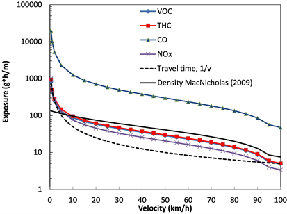
Figure 9. Pollution exposure per length as function of traffic flow velocity.

Figure 10. Plot showing contribution to exposure by a road segment.

Figure 11. Relative size of total exposure per vehicle .
Figure 11 show the segment’s contribution to total exposure per unit length is in terms of that is the total contribution to exposure per unit square length for time spent on the segment. Policies reflected by authority regulations are in Norway given as an annual (or winter) average maximum value of pollution concentration at 2 - 3 m height above the ground. A yellow limit for NO2 is 40 μg/m3 winter averages and a red limit is 40 μg/m3 annual averages [43] . Comparing Figure 8 and Figure 9, it is seen that increasing the velocity or capacity of roads from congested velocities of 25 km/h to 65 - 70 km/h, would keep the concentration about constant but reduce health risk by 50% and be Pareto optimal [44] .
Traffic map companies have developed methods to predict future or typical traffic based on current and historic traffic. The future traffic can be predicted on a short-term basis, typical one hour. By combining smartphone trajectory, this traffic prediction can be used to predict the next hour exposure for a given planned route. It would then be straight forward to compare several possible routes and make an intelligent choice based on weighting “time to target location” versus “pollution exposure to target location” and optimize the route based on individual preferences.
Traffic is well-known to display certain typical patters. Large cities have a typical daily M-shaped density peak of morning and afternoon rush hours due to the flow of commuters in and out of the city. The peak sizes vary typically with weekdays. This information can be used in projecting future long term exposure, identify high exposure groups and check if negative health impact is well-correlated to high exposure groups.
Further one may use the prediction or average maps to estimate where the future population health risk is highest and direct infrastructure investments to minimize a combination of “population travel time” and “population health risk”. Our modelling of exposure showed that the high exposure at low velocity scales as and this correlates well to the traffic map itself, since a small gives both high exposure and congestion. Most people travel on the peaks of the M-shaped rush hour peaks it is clear that just reducing the size of the rush hour peaks would lead to a significantly improved population health. Exposure maps and health risk maps could be a highly useful tool for urban planning of transport infrastructure in interaction to where people live and work. Even more useful for predictions would be to develop urban simulators where every person in the city have simulated trajectories and would then get simulated exposures and health risks. An urban simulator could then be used to answer all kinds of “what if” questions. An urban simulator could be a highly valuable tool for politicians and urban planners. We predict that by 2030 urban trajectory simulators are routinely being applied in urban planning.
4. Conclusions
It is feasible to combine traffic maps data with smartphone location service trajectories and big data analytics to simulate near real-time traffic air pollution exposure and health risk. Advantages of the approach are: i) low cost, ii) near real-time, iii) effortless citizen participation, and iv) global scalability.
Nearly every modeling step of traffic air pollution depends on traffic velocity. A traffic map is a super-efficient pre-processor for calculating real-time traffic pollution.
Universally, the exposure and health risk has a peak at lower velocities than the peak of concentration. Congestion is a higher health risk than conventionally believed.
Acknowledgements
We thank Mr. Mike Kobernus at NILU (Norwegian Institute for Air Research) for help with the language. Any remaining errors are the responsibility of the authors.
Cite this paper
Skjetne, E. and Liu, H.-Y. (2017) Traffic Maps and Smartphone Trajectories to Model Air Pollution, Exposure and Health Impact. Journal of Environmental Protection, 8, 1372-1392. https://doi.org/10.4236/jep.2017.811084
References
- 1. Vidal, J. (2010) UN Report. World’s Biggest Cities Merging into “Mega-Regions”. http://www.theguardian.com/world/2010/mar/22/un-cities-mega-regions
- 2. CITEAIR (2007) EU: Air Quality in Europe—Pollution Basics. http://www.airqualitynow.eu/pollution_home.php
- 3. Moscow Pilot Methodogical Geochemical Expedition of Institute of Mineralogy, Geochemistry and Crystallochemistry (1996-1998) The ENVIBASE-Project: Chapter 3—Traffic—Moscow. http://www.stadtentwicklung.berlin.de/archiv_sensut/umwelt/uisonline/envibase/handbook/traffic4.htm
- 4. TomTom. (2013) TomTom Congestion Index Shows That Moscow Is the Most Congested City. http://corporate.tomtom.com/releasedetail.cfm?ReleaseID=754227
- 5. Rank, J., Folke, J. and Jespersen, P.H. (2001) Differences in Cyclists and Car Drivers’ Exposure to Air Pollution from Traffic in the City of Copenhagen. Science of the Total Environment, 279, 131-136. https://doi.org/10.1016/S0048-9697(01)00758-6
- 6. van Wijnen, J.H., Verhoeff, A.P., Jans, H.W. and van Bruggen, M. (1995) The Exposure of Cyclists, Car Drivers and Pedestrians to Traffic-Related Air Pollutants. International Archives of Occupational and Environmental Health, 67, 187-193. https://doi.org/10.1007/BF00626351
- 7. Brauer, M., Reynolds, C. and Hystad, P. (2012) Traffic-Related Air Pollution and Health: A Canadian Perspective on Scientific Evidence and Potential Exposure-Mitigation Strategies. Report for Water, Air and Climate Change Bureau, Health Canada. University of British Columbia, Vancouver, BC.
- 8. HEI Panel on the Health Effects of Traffic-Related Air Pollution (2010) Traffic-Related Air Pollution: A Critical Review of the Literature on Emissions, Exposure, and Health Effects. Boston, Massachusetts.
- 9. US EPA (2017) How Mobile Source Pollution Affects Your Health. http://www3.epa.gov/otaq/nearroadway.htm
- 10. King’s Colleague London (2017) London Air—Mobile Apps. http://www.londonair.org.uk/LondonAir/MobileApps
- 11. U.S. EPA. Air Now. http://www.airnow.gov/
- 12. Castell, N., Liu, H.-Y., Schneider, P., Cole-Hunter, T., Lahoz, W. and Bartonova, A. (2015) Towards a Personalized Environmental Health Information Service Using Low-Cost Sensors and Crowdsourcing. Geophysical Research Abstracts, 17, EGU2015-9058.
- 13. Reisa, S., Seto, E., Northcross, A., Quinn, N.W.T., Convertino, M., Jones, R.L., Maier, H.R., Schlink, U., Steinle, S., Vieno, M. and Wimberly, M.C. (2015) Integrating Modelling and Smart Sensors for Environmental and Human Health. Environmental Modelling & Software, 74, 238-246. https://doi.org/10.1016/j.envsoft.2015.06.003
- 14. US EPA (2017) Air Sensor Toolbox for Citizen Scientists, Researchers and Developers. http://www2.epa.gov/air-research/air-sensor-toolbox-citizen-scientists
- 15. CITI-SENSE Consortium (2012-2016) CITI-SENSE—Development of Sensor-Based Citizens’ Observatory Community for Improving Quality of Life in Cities. http://co.citi-sense.eu
- 16. EveryAware Consortium (2012-2015) EveryAware—Enhance Environmental Awareness through Social Information Technologies. http://www.everyaware.eu
- 17. iSPEX Consortium (2015) iSPEX—Measure Aerosols with Your Smartphone. http://ispex.nl/en
- 18. Brienza, S., Galli, A., Anastasi, G. and Bruschi, P. (2015) A Low-Cost Sensing System for Cooperative Air Quality Monitoring in Urban Areas. Sensors, 15, 12242-12259. https://doi.org/10.3390/s150612242
- 19. Piedrahita, R., Xiang, Y., Masson, N., Ortega, J., Collier, A., Jiang, Y., Li, K., Dick, R., Lv, Q., Hannigan, M. and Shang, L. (2014) The Next Generation of Low-Cost Personal Air Quality Sensors for Quantitative Exposure Monitoring. Atmospheric Measurement Techniques Discussions, 7, 2425-2457. https://doi.org/10.5194/amtd-7-2425-2014
- 20. Liu, H.-Y., Skjetne, E. and Kobernus, M. (2013) Mobile Phone Tracking: In Support of Modelling Traffic-Related Air Pollution Contribution to Individual Exposure and Its Implications for Public Health Impact Assessment. Environmental Health, 12, 93. https://doi.org/10.1186/1476-069X-12-93
- 21. Liu, H.-Y., Kobernus, M., Broday, D. and Bartonova, A. (2014) A Conceptual Approach to a Citizens’ Observatory—Supporting Community-Based Environmental Governance. Environmental Health, 13, 107. https://doi.org/10.1186/1476-069X-13-107
- 22. US EPA (2017) Emission Facts Idling Vehicle Emissions for Passenger Cars, Light-Duty Trucks, and Heavy-Duty Trucks. http://www.epa.gov/otaq/consumer/420f08025.pdf
- 23. Cobb, J. (2016) Top Six Plug-In Vehicle Adopting Countries—2015. http://www.hybridcars.com/top-six-plug-in-vehicle-adopting-countries-2015
- 24. Google (2017) View Traffic, Satellite, Terrain, Biking, and Transit. https://support.google.com/maps/answer/3093389?rd=1
- 25. Wikipedia (2017) Traffic Flow. https://en.wikipedia.org/wiki/Traffic_flow
- 26. Wikipedia (2008) Fundamental Diagram of Traffic Flow. http://en.wikipedia.org/wiki/Fundamental_diagram_of_traffic_flow
- 27. Yandex (2017) Yandex Traffic Jam Technology Overview. http://company.yandex.com/technologies/traffic_jams_technology.xml
- 28. Guo, Z. (2013) How Google Tracks Traffic. https://wagner.nyu.edu/node/22485
- 29. Wikipedia (2016) Fundamentals of Transportation/Traffic Flow. http://en.wikibooks.org/wiki/Fundamentals_of_Transportation/Traffic_Flow
- 30. Transportation Research Board of the National Academics (2011) 75 Years of the Fundamental Diagram for Traffic Flow Theory. Transportation Research Board, Washington DC.
- 31. Van Aerde, M. (1995) Single Regime Speed-Flow-Density Relationship for Congested and Uncongested Highways. Proceedings of the 74th TRB Annual Conference, Washington DC, 27 January 1995, Paper No. 950802.
- 32. MacNicholas, M.J. (2011) A Simple and Pragmatic Representation of Traffic Flow. Proceedings of the Greenshields Symposium on 75 Years of the Fundamental Diagram for Traffic Flow Theory, Washington DC, 7-10 July 2008, 161-177.
- 33. Kerner, B.S. (1998) Experimental Features of Self-Organization in Traffic Flow. Physical Review Letters, 81, 3797. https://doi.org/10.1103/PhysRevLett.81.3797
- 34. Bellander, T., Berglind, N., Gustavsson, P., Jonson, T., Nyberg, F., Pershagen, G. and Järup, L. (2001) Using Geographic Information Systems to Assess Individual Historical Exposure to Air Pollution from Traffic and House Heating in Stockholm. Environmental Health Perspectives, 109, 633-639. https://doi.org/10.1289/ehp.01109633
- 35. Luhar, A.K. and Patil, R.S. (1989) A General Finite Line Source Model for Vehicular Pollution Prediction. Atmospheric Environment, 23, 555-562. https://doi.org/10.1016/0004-6981(89)90004-8
- 36. NVIDIA (2009) Real Time 3D Fluid and Particle Simulation and Rendering. https://www.youtube.com/watch?v=RuZQpWo9Qhs
- 37. Wikipedia (2017) Density. http://en.wikipedia.org/wiki/Density
- 38. Kim, Y. (2011) Quantification of Vehicle-Induced Turbulence on Roadways Using Computational Fluid Dynamics Simulation. Master Thesis, University of Toronto, Toronto.
- 39. Davidson, G.A. (1990) A Modified Power Law Representation of the Pasquill-Gifford Dispersion Coefficients. Journal of the Air & Waste Management Association, 40, 1146-1147. https://doi.org/10.1080/10473289.1990.10466761
- 40. Green, A.E., Singhal, R.P. and Venkateswar, R. (1980) Analytic Extensions of the Gaussian Plume Model. JAPCA, 30, 773-776. https://doi.org/10.1080/00022470.1980.10465108
- 41. Integrated Assessment Toolbox Consortium (2005-2011) Time Micro-Environment Activity Modelling. http://www.integrated-assessment.eu/node/204
- 42. Wikipedia (2017) Taylor Series. http://en.wikipedia.org/wiki/Taylor_series
- 43. Gulia, S., Nagendra, S.M.S., Khare, M. and Khanna, I. (2015) Urban Air Quality Management—A Review. Atmospheric Pollution Research, 6, 286-304. https://doi.org/10.5094/APR.2015.033
- 44. Wikipedia (2017) Pareto Optimal. http://en.wiktionary.org/wiki/Pareto_optimal