Journal of Environmental Protection
Vol. 3 No. 10 (2012) , Article ID: 23866 , 10 pages DOI:10.4236/jep.2012.310152
Non-Homogeneous Poisson Processes Applied to Count Data: A Bayesian Approach Considering Different Prior Distributions
![]()
1Department of Statistics, Federal University of Santa Maria, Santa Maria, Brazil; 2Department of Statistics, University of Campinas, Campinas, Brazil; 3Department of Social Medicine, Medical School, University of São Paulo, Ribeirão Preto, Brazil.
Email: *hotta@ime.unicamp,br
Received July 22nd, 2012; revised August 21st, 2012; accepted September 23rd, 2012
Keywords: Non-Homogeneous Poisson Processes; Bayesian Analysis; Markov Chain Monte Carlo Methods and Simulation; Prior Distribution
ABSTRACT
This article discusses the Bayesian approach for count data using non-homogeneous Poisson processes, considering different prior distributions for the model parameters. A Bayesian approach using Markov Chain Monte Carlo (MCMC) simulation methods for this model was first introduced by [1], taking into account software reliability data and considering non-informative prior distributions for the parameters of the model. With the non-informative prior distributions presented by these authors, computational difficulties may occur when using MCMC methods. This article considers different prior distributions for the parameters of the proposed model, and studies the effect of such prior distributions on the convergence and accuracy of the results. In order to illustrate the proposed methodology, two examples are considered: the first one has simulated data, and the second has a set of data for pollution issues at a region in Mexico City.
1. Introduction
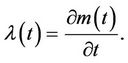
The non-homogeneous Poisson model has been applied to various situations, such as the analysis of software reliability data, air pollution data and medical count data. Denote by M(t) the cumulative number of events in the time interval (0, t] for t ≥ 0. M(t) is modelled by a non-homogeneous Poisson process with mean value function m(t). The mean value function m(t) changes according to the model, i.e., it assumes the shape of the distribution that is being used. One can also characterize the distribution by the intensity function
If λ(t) is a constant, so that m(t) is linear, then M(t) is called a homogeneous Poisson process; otherwise the process is called a non-homogeneous Poisson process.
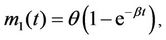
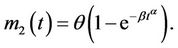
Many different choices for the function m(t) are considered in the literature, especially in software reliability [1]. Reference [2] considered that the expected number of software failures for time t, given by the mean value function m(t), is non-decreasing and bounded above. Specifically, they have considered the mean function
 (1)
(1)
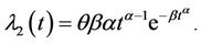
where θ, in our application represents the expected maximum number of days in which air quality standard is violated by a particular pollutant and β the rate at which events occur. By (1), we have that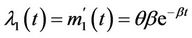 . In [3] a generalization of the model given by (1) was proposed, with the following intensity function
 (2)
(2)
The corresponding mean function is
 (3)
(3)
Note that (1) and (3) can be written as special cases of the general form where the mean value function is given as
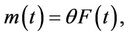 (4)
(4)
where F(t) is a distribution function. On the other hand, for any distribution function F(t) we have a valid model. A widely used distribution function, given its high flexibility of fit, is the Generalized Gamma distribution. In this case the mean function is
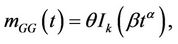 (5)
(5)
where Ik(s) is the integral of the Gamma function given by
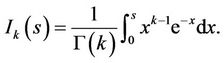 (6)
(6)
From Equation (6), we obtain the intensity function given by
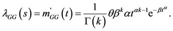 (7)
(7)
This model is called Generalized Gamma model. When k is integer we can write F(t) as
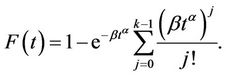 (8)
(8)
The three models used in this article are described as follows:
1) Model I: Here all the parameters are unknown, and λGG(t) is given by (7);
2) Model II: with k = 1, λGG(t) is given by the function λ2(t) given in (2) [3];
3) Model III: with k = 1 and α = 1, λGG(t) reduces to λ1(t) [2].
It is important to point out that other generalized models could be considered in this case. A particular case is given by the exponentiated-Weibull distribution (see, for example, [4-6]). This model permits bathtub forms for the intensity function, besides the forms assumed by the Generalized Gamma distribution. This case is beyond the goals of this paper.
In the Bayesian analysis of Models I, II and III, we may have some difficulties in obtaining the Bayesian inferences using MCMC simulation methods. In order to do so, let us study the effect of different prior distributions on the performance of sample simulation algorithms for the posterior distribution in which we are interested.
The focus of this paper is to propose different prior distribution specifications for the parameters, because when we consider the models with all parameters being free and to be estimated, we found some convergence problems in the MCMC algorithm for simulating samples of the joint posterior distribution. Therefore, a sensitivity analysis of the estimation of the parameters of the models is conducted which relates to the choice of prior distributions. The biggest concern is with the parameter k, a parameter of the Gamma distribution [5].
In this article we will present two prior distribution proposals for the parameter k of the Generalized Gamma model. The first uses the prior distributions for the parameters used in [1]. Given the problems with this prior, especially of convergence of the Gibbs sampling algorithm, a second prior distribution is suggested for the parameter k, which is a truncated exponential distribution. As we shall see, this distribution proves to be adequate. Other distributions were tested, but will not be displayed. We chose to present only the two assumed prior distributions, because the first one is suggested in the literature and the second one has shown good results.
The convergence of the MCMC algorithm was analysed by graphical methods and by the Gelman-Rubin criterion. The Gelman-Rubin criterion [7] relies on parallel chains to test whether they all converge to the same posterior distribution. In [8] the introduction of a correction factor was suggested. This corrected statistics was evaluated using the CODA package in R. The closer this statistics is to 1.0, the more evidence we have that the chain is near convergence. The limit value of 1.2 is sometimes used as a guideline for “approximate convergence” [9].
This article is structured as follows. In Section 2 we present the Bayesian inference for the models discussed here. Section 3 introduces an example of this process with simulated data, and we use the two prior distributions mentioned previously for the parameter k. An application to Mexico City’s pollution data is performed in Section 4. In Section 5 some concluding remarks are made.
2. Bayesian Inference
The data set is denoted by DT = {n; t1, t2, ···, tn; T}, where n is the number of events observed such that 0 ≤ t1 ≤ t2 ≤ ··· ≤ tn ≤ T, and ti are the times of the events observed during the period of time (0, T].
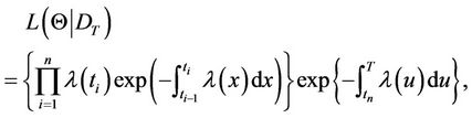
The likelihood function for the vector 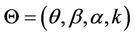 considering the truncated time of the model (see, for example, [10]) is given by
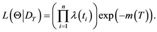 (9)
(9)
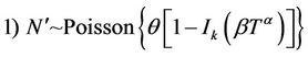
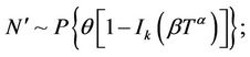
In some cases it is necessary to introduce a latent variable; this latent variable may improve the convergence of the MCMC algorithm. We considered the introduction of a latent variable N’ that has Poisson distribution with parameter 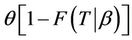 (see [1] for details).
Considering the mean function (5) with a Generalized Gamma distribution, the likelihood function for the parameters θ, β, α and k is expressed as
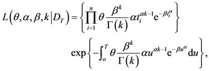
such that,
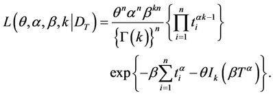 (10)
(10)
2.1. Prior Distributions
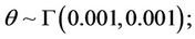
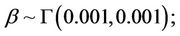
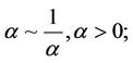
The first set of prior distributions for the general Model I are the distributions suggested by [1]:
 ;
;
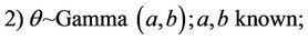
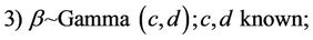
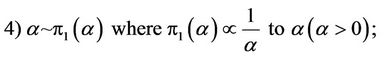
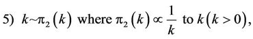
where P(λ) denotes the Poisson distribution with parameter λ. Observe that the prior distributions for k and α are improper priors. With this choice of prior distribution we cannot guarantee that for all data sets the posterior distribution is proper; in other words, we could have convergence problems in the simulation algorithm for samples of the joint posterior distribution. To overcome this problem, we assume a truncated exponential prior for k, but other priors could be used as the Gamma distribution. This is a subject of a future work. Thus, in the second set, also for the general Model I, we assume other prior specifications for the parameters α and k, i.e., given by
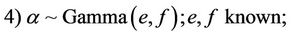

where a, b, c, d, e, f and an are the known hyperparameters of the gamma distribution where Γ(a, b) denotes a gamma distribution with mean  and variance
 .
.
Further, let us assume prior independence among the parameters. The values of the hyperparameters are given in the applications, following expert opinion or even from some information in the data (use of empirical Bayesian methods). As we have convergence problems in the chains of the parameter k, the effects of other priors for this parameter are studied in the applications. These priors distributions are given in Section 3.
In the restricted Models II and III the same prior distributions are used for the free parameters.
2.2. Posterior Distributions
The inference will be conducted based on information supplied by the posterior distribution of the parameters. From the Bayes formula, the joint posterior distribution is obtained by combining the prior and the likelihood function. The likelihood function for homogeneous or non-homogeneous Poisson processes is given by,
or 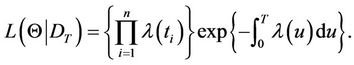
Thus, we have
 (11)
(11)
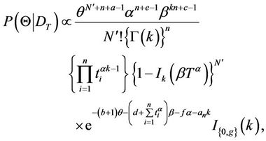
Initially we will consider the case where the prior distribution of k is that suggested by [1]. In this case, the posterior distribution is given by
 (12)
(12)
Because the posterior distribution in (12) has no closed form, we resort to MCMC methods to generate samples for the joint posterior distribution. The algorithm used to obtain posterior distribution samples in (12) is given as follows. For the subset of parameters whose full conditional density is known, we simulate samples directly from these distributions, using the Gibbs Sampling algorithm; for the set of parameters whose conditional densities are not known standard densities, the samples are taken using the steps of the Metropolis-Hastings algorithm [11,12]. Recommended references for a review of the MCMC methods are given in [13].
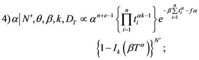
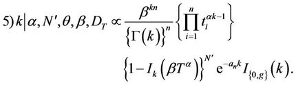
The conditional posterior distributions required for MCMC methods are given by
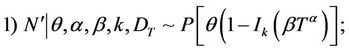
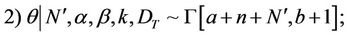
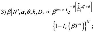
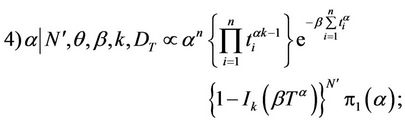
The distribution for the parameter θ has a closed form distribution, so the posterior distributions of θ are obtained through the Gibbs sampling method. Since the posterior distributions of α, β and k do not have a closed form, we resort to MCMC methods to simulate samples of these random quantities. The algorithm used to obtain posterior distribution samples of the parameters α, β and k, whose full conditional densities are not known, is the Metropolis-Hastings algorithm.
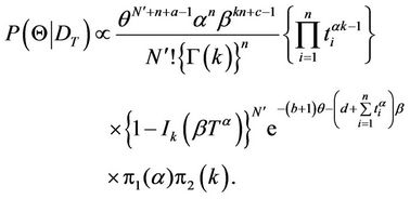
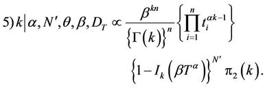
When we adopt the prior specification of the second set, proposed in Model I, we have that the posterior distribution is given by
 (13)
(13)
and the only changes in the marginal posterior densities occur in 4) and 5), which are replaced by
3. A Simulated Study
In this section we use a set of simulated data with a sample size of 300 observations with θ = 300, β = 0.02, α = 1 and k = 1.
For both sets 1 and 2 of the prior specifications of Model I we found problems of convergence of the Gibbs sampling algorithm for all parameters. We used a burn-in of 15,000 iterations to eliminate the effects of the initial values, and after the burn-in period another 900,000 iterations were simulated. Taking every 500th step, which gives a final sample of size 1800 we obtained Monte Carlo estimates for the random quantities of interest.
We also obtained posterior estimates of the restricted models: Model II, k = 1 and Model III, k = 1, α = 1. We used a burn-in of 50,000 iterations, and after this we obtained 5000 samples of the posterior distributions, a sample at each tenth iteration.
In Model I, assuming set 1 of the priors of [1], we have,
Let us call the model with this prior specification as Model I(1).
In Model I with the second set of prior specifications, we assume a Gamma prior distribution for α given by Γ(0.001, 0.001). For the parameter k we conducted a study of the sensitivity of different priors assuming different hyperparameter values. This was done because, when this parameter is estimated, it is difficulty to obtain convergence of the algorithm used to simulate samples for the parameters. The prior distributions tested for this parameter include: Uniform (0, T), Γ(0.001, 0.001) and Γ(10,000), besides other values for the hyperparameters of such distributions. The transformation log(k) was also tested, where log(K) ~ N(a1, b1), with many values for the hyperparameters a1, b1, including N(0, 0.01), N(10, 10) and N(0, 1). In most tests the convergence of the Markov chain simulations was not satisfactory. The best result was obtained for a truncated exponential distribution with mean parameter equal to 0.95 and truncated in 3. Let us call the model with this prior distribution Model I(2). Table 1 shows summaries of the posterior the estimates of Models I, II and III.
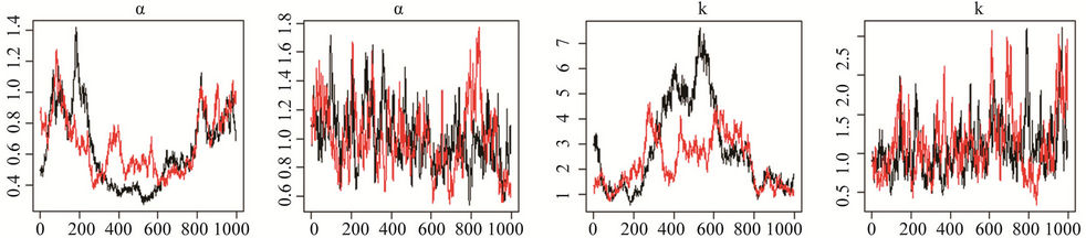
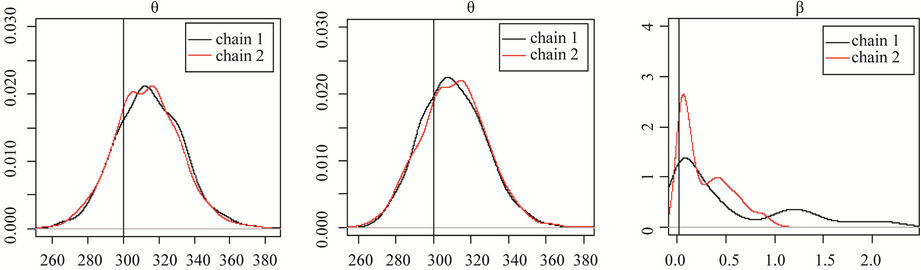
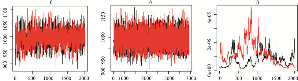
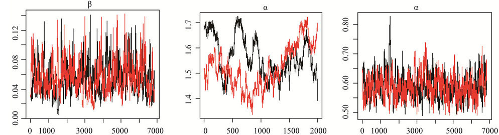
For Model I(1) which uses a non-informative prior distribution specification for parameter k, the graphs of the MCMC chains are shown in Figure 1 (letters (a), (c), (e) and (g)). Only for parameter θ (letter (a)) do we appear to have clear convergence, while for the parameter β (letter (c)) there is clear nonconvergence, and for parameter k (letter (g)) there is possible nonconvergence. Figure 2 (letters (a), (c), (e) and (g)) presents the posterior distributions of the two chains. Only for the parameter θ (letter
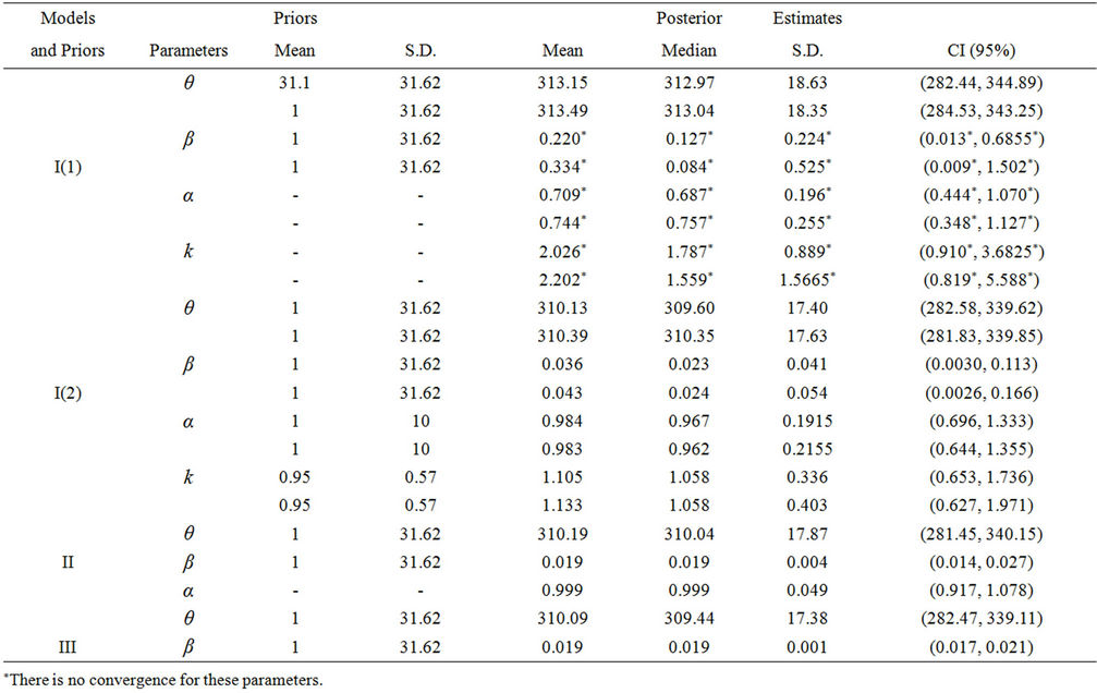
Table 1. Posterior summaries of the estimates of the parameters for Models I, II and III. True model: θ = 300, β = 0.02, α = 1 and k = 1. Sample size of 300. Priors: for the parameters θ, β and α the prior distributions are the ones in Section 2. For the parameter in Model I: (1) Non-informative prior distribution proposed in [1]; (2) Exponential prior distribution with mean parameter 0.95 and truncated in 3. For Model I, we have: 1st row of each parameter corresponds to an estimate of chain 1, starting from a given value; 2nd row corresponds to an estimate of chain 2, starting from the true values.

(a)(b)(c)(d) (e)(f)(g)(h)
Figure 1. Convergence of chains 1 and 2, for the parameters of Model I(1), for which the graphs are labeled (a), (c), (e) and (g), and Model I(2), for which the graphs are labeled (b), (d), (f) and (h).

(a)(b)(c) (d)(e)(f) (g)(h)
Figure 2. Posterior distribution of the parameters for chains 1 and 2 of Model I, where graphs (a), (c), (e) and (g) correspond to the first set of priors, and graphs (b), (d), (f) and (h) correspond to the second set of priors. The true value of each parameter is represented by a vertical line.
(a)) is there any indication of convergence. These results are confirmed by the Gelman-Rubin’s statistics which are equal to 1.25 and 1.15, for the parameters β and k respectively. That is, we did not get convergence for the MCMC chains with these prior distributions.
In Model I(2) we use, as the new proposed prior distribution for the parameter k, an exponential distribution with mean parameter 0.95 and truncated in 3. The chains are presented in Figure 1 (letters (b), (d), (f) and (h)) and there is an indication of convergence. Figure 1 (letters (b), (d), (f) and (h)) shows the posterior distribution of the parameters for chains 1 and 2, and there is also indication of convergence. The convergence is confirmed by the Gelman-Rubin’s statistics, with the largest value equal to 1.01.
The main conclusion reached in this sensitivity analysis is that in the case of the proposed Model 2, this is close to the process that generates the actual data; in other words, it is possible to have a good approximation of the posterior distribution of the parameters. Even using prior distributions for parameters α, β and θ which are not very informative, Model I(2) can estimate the true value of these parameters. This does not hold true for Model I(1).
4. An Application to Pollution Data
This section applies Models I(1) and I(2) to fit data corresponding to the maximum daily mean measurements of ozone gas, based on data from the northeast (NE) region of Mexico City. The sample has 981 observations, which correspond to times when a certain threshold established for the air quality standard is violated in the interval time (0,T] These data are available at www.sma.df.gob.mx/simat, and we took eighteen years of observations, from January 1st, 1990 to December 31st, 2008 [14].
For these models and the assumed data set we used a burn-in of 15,000 iterations, and after this we obtained 7000 samples of the posterior distributions, with a sample at each one-hundredth iterations.
Table 2 shows the posterior estimates of the parameters for Models I(1) and I( 2).
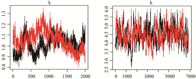
In Figure 3, we show the trace plots of chains 1 and 2, respectively, for the parameters of the models, where graphs (a), (c), (e) and (g) correspond to Model I(1), and graphs (b), (d), (f) and (h) correspond to Model I(2). We can observe in Figure 3, that in graphs (a), (c), (e) and (g), related to Model I(1), only parameter θ appears to have convergence (graph (a)), and there is evidence that there is non convergence for the other parameters. In this model we used a non-informative prior distribution specification for the parameter k. In Model I(2), graphs (b), (d), (f) and (h), appear to have convergence. In this model we proposed as the prior distribution for the parameter k an exponential distribution with mean parameter 0.99 and truncated in 6.
The largest value of the Gelman-Rubin’s statistics for the parameters of the general Model I(2) is equal to 1.00 indicating convergence of the MCMC chains. In Model I(1) the Gelman-Rubin’s statistics are equal to 1.22, 1.23 and 1.19, for the parameters α, β and k respectively. So we did not get the convergence of the MCMC chains using the non informative prior for the parameter k.
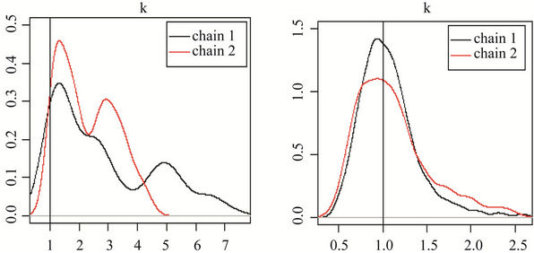
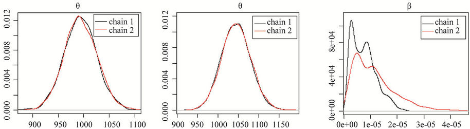
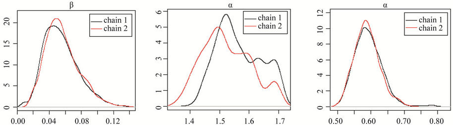
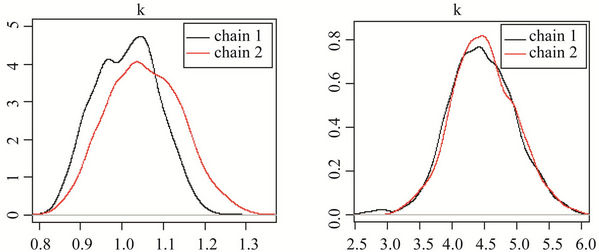
In Figure 4, we have the posterior distribution of the parameters for chains 1 and 2 for Models I(1) and I(2). The graphs labelled (a), (c), (e) and (g) correspond to the first set of priors; and the graphs t labelled (b), (d), (f)
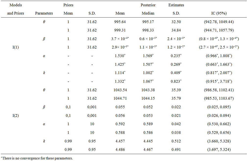
Table 2. Posterior estimates of parameters, using a sample of real data corresponding to the NE region of Mexico City. Priors: for parameters θ, β and α the prior distributions are the ones in Section 2. Priors for parameter k: Model I(1) non-informative prior distribution proposed in [1]; Model I(2) exponential prior distribution with mean parameter 0.99 truncated in 6. In the 1st row, for each parameter, we present the estimates corresponding to chain 1, and in the 2nd row, we present estimates corresponding to chain 2.
(a)(b)(c) (d)(e)(f) (g)(h)
Figure 3. Convergence of chains 1 and 2, for the parameters of Model I(1), in which the graphs are labelled (a), (c), (e) and (g), and Model I(2), in which the graphs are labelled (b), (d), (f) and (h).
and (h) correspond to the second set of priors. The results confirm the convergence in the Model I(2) and nonconvergence in Model I(1)
5. Conclusions
In this article we proposed a sensitivity analysis with various specifications of prior distributions for the model previously introduced in [1], which was developed using the Bayesian approach. We have conducted a study of the effect of prior distributions on the convergence and accuracy of the results, and in this way we have been able to propose a prior distribution for the parameter k that gives convergence of the samples simulation algorithm. Observe that using improper prior distributions for the parameter k could not guarantee that the posterior distribution was proper, as this depended on the data set (as was observed in our application with real data). After trying several prior distribution specifications for this parameter, it was possible to propose a prior distribution that would considerably improve the convergence of the chains. Such improvements can be noted in credible intervals, in which the range of the interval is smaller using a truncated exponential prior distribution; we may also observed these best results through graphical analysis when using a truncated exponential prior distribution for the parameter k, we obtained convergence of the chains.
It is important to point out that other informative priors
(a)(b)(c) (d)(e)(f) (g)(h)
Figure 4. Posterior distributions of parameters for chains 1 and 2, respectively for Model I, where graphs (a), (c), (e) and (g), correspond to the first set of priors and graphs (b), (d), (f) and (h) correspond to the second set of priors.
for the parameter k could be considered, such as a Gamma distribution. This possibility is a goal for a future study.
6. Acknowledgements
This work was partially supported by grants from Capes, CNPq and FAPESP. We would like to thank one referee and Laboratório Epifisma.
REFERENCES
- J. A. Achcar, K. D. Dey and M. Niverthi, “A Bayesian Approach Using Nonhomogeneous Poisson Process for Software Reliability Models,” In: A. S. Basu, S. K. Basu and S. Mukhopadhyay, Eds., Frontiers in Reliability, World Scientific Publishing Co., Singapore City, 1998, pp. 1-18. doi:10.1142/9789812816580_0001
- A. L. Goel and K. Okumoto, “An Analysis of Recurrent Software Errors in a Real-Time Control System,” Proceedings of the 1978 Annual Conference, ACM’78, Washington DC, 4-6 December 1978, pp. 496-501. doi:10.1145/800127.804160
- A. L. Goel, “A Guidebook for Software Reliability Assessment,” Technical Report, Syracuse University, Syracse, 1983.
- G. S. Muldholkar, D. K. Srivastava and M. Friemer, “The Exponentiated-Weibull Family: A Reanalysis of the BusMotor Failure Data,” Technometrics, Vol. 37, No. 4, 1995, pp. 436-445. doi:10.1080/00401706.1995.10484376
- V. G. Cancho, H. Bolfarine and J. A. Achcar, “A Bayesian Analysis of the Exponentiated-Weibull Distribution,” Journal of Applied Statistical Science, Vol. 8, No. 4, 1999, pp. 227-242.
- J. E. R. Cid and J. A. Achcar, “Bayesian Inference for Nonhomogeneous Poisson Processes in Software Reliability Models Assuming Nonmonotonic Intensity Functions,” Computational Statistics and Data Analysis, Vol. 32, No. 2, 1999, pp. 147-159. doi:10.1016/S0167-9473(99)00028-6
- A. Gelman and D. R. Rubin, “A Single Series from the Gibbs Sampler Provides a False Sense of Security,” In: J. M. Bernardo, J. O. Berger, A. P. Dawid and A. F. M. Smith, Eds., Bayesian Statistics 4, Oxford University Press, Oxford, 1992, pp. 625-631.
- S. P. Brook and A. Gelman, “General Methods for Monitoring Convergence of Iterative Simulations,” Journal of Computational and Graphical Statistics, Vol. 7, No. 4, 1997, pp. 434-455. doi:10.2307/1390675
- A. Gelman, “Inference and Monitoring Convergence,” In: W. R. Gilks, S. Richardson and D. J. Spiegelhalter, Eds., Markov Chain Monte Carlo in Practice, Chapman and Hall, London, 1996, pp. 131-143.
- D. R. Cox and P. A. Lewis, “Statistical Analysis of Series of Events,” Methuen, London, 1966. doi:10.1063/1.1699114
- N. Metropolis, A. W. Rosenbluth, M. N. Rosenbluth, A. H. Teller and E. Teller, “Equations of State Calculations by Fast Computing Machines,” Journal of Chemical Physics, Vol. 21, No. 6, 1953, pp. 1087-1092. doi:10.1063/1.1699114
- W. K. Hastings, “Monte Carlo Sampling Methods Using Markov Chains and Their Applications,” Biometrika, Vol. 57, No. 1, 1970, pp. 97-109. doi:10.1093/biomet/57.1.97
- G. Casella, and R. L. Berger, “Statistical Inference,” 2nd Edition, Duxbury Press, Pacific Grove, 2001.
- J. A. Achcar, E. R. Rodrigues, C. D. Paulino and P. Soares, “Non-homogeneous Poisson Models With a Change-Point: An Application to Ozone Peaks in Mexico City,” Environmental and Ecological Statistics, Vol. 17, No. 4, 2010, pp. 521-541. doi:10.1007/s10651-009-0114-3
NOTES
*Corresponding author.