Atmospheric and Climate Sciences
Vol. 2 No. 1 (2012) , Article ID: 17128 , 16 pages DOI:10.4236/acs.2012.21008
Analysis of Winds Affecting Air Pollutant Transport at La Plata, Argentina
1CIOp (Centro de Investigaciones Ópticas), La Plata, Argentina
2Facultad de Ingeniería, Universidad Nacional de La Plata, La Plata, Argentina
3Facultad de Ciencias Exactas, Departamento de Matemáticas, Universidad Nacional de La Plata, La Plata, Argentina
4Facultad de Fisicomatemáticas e Ingeniería y Facultad de Ciencias Agrarias, Pontificia Universidad Católica Argentina, Buenos Aires, Argentina
5Universidad Tecnológica Nacional (UTN), Facultad Regional Buenos Aires, Buenos Aires, Argentina
6CIC BA (Comisión de Investigaciones Científicas de la Pcia. de Buenos Aires), La Plata, Argentina
7Centro Agrario El Chaparillo, Junta de Comunidades de Castilla La Mancha, Ciudad Real, España
8Universidad Tecnológica Nacional (UTN), Facultad Regional La Plata, La Plata, Argentina
Email: *gustavratto@gmail.com
Received October 4, 2011; reivsed December 5, 2011; accepted December 29, 2011
Keywords: La Plata; Local Smoothing; Minimum Covariance Determinant; Robust Correlation; Similarity; Wind Analysis
ABSTRACT
An hourly wind analysis for the populated area of La Plata city (with high industrial, power station and vehicular activities) is presented and discussed. Euclidean distance and minimum covariance determinant (a robust correlation coefficient) are employed, as similarity approaches, in order to compare observed wind direction frequency patterns at two monitoring sites during 1998-2003. A preliminary assessment of two sectors, namely Sector 1 (NNW-N-NNE-NE) and Sector 2 (ENE-E-ESE), relevant for the transport of industrial air pollutants towards population exposed, is discussed taking variances into account and employing a locally weighted smoothing approach (LOESS). Both similarity approaches allowed gain insight of wind patterns. The distance approach showed good similarity between sites while the correlation approach showed an uneven picture depending on the wind direction. Most of the differences are explained in terms of the sea-land breeze effect but also differences in terrain roughness and data quality are taken into account. Winds from sectors 1 or 2 (analyzed during 1998-2009) may occur more than 50% of the time, most of the differences regarding the influence of the day and the season on these sectors are attributable to sea-land breeze phenomena. The LOESS proved to be appropriate to analyze the stability with time of both sectors and to discard possible remaining patterns; results are in accordance with studies that assess the interannual variability for different variables in La Plata river area. The robust correlation coefficient revealed, as an example, the linear character of dependence between winds from sector 2 and sulfur dioxide concentrations. Wind velocities and calms are also discussed.
1. Introduction
Urban areas are major sources of air pollution which is the result of processes of accumulation, dispersion, transformation and removal of contaminants. Pollutant emissions affecting air quality in cities have an adverse impact on human health [1]. The city of La Plata and its surroundings are densely populated areas (approximately 800,000 inhabitants) with high industrial and vehicular activity. Glassmann and Mazzeo [2] made a regional study of air pollution potential in Argentina and concluded that La Plata is located in a zone with poor atmospheric self-cleansing capacity. In spite of these facts, no governmental air monitoring network is installed. In recent years several works contributed to assess different parameters characterizing air pollutants in the area [3-7] but references to hourly distribution of winds and sealand breeze effects have been rare. The characterization of wind direction frequency patterns associated with industrial sources is essential for describing the transporttation of air pollutants and settles the basis for a further assessing of environmental impact on human health.
Enriching previous reports this article make available a detailed summary of wind direction frequencies while discusses their importance for air pollutant modeling.
One purpose of this paper is to compare observed wind direction frequency patterns covering the period 1998- 2003 at two monitoring sites (named Point A and J Figure 1). A previous report [8] analyzed similarity between both sites employing cluster and multidimensional scaling analysis. The present study is intended to gain insight of hourly occurrences of winds regarding air pollutants. To this end two different approaches are involved: one quantifies proximity using the squared Euclidean distance and the other quantifies correlation applying to the minimum covariance determinant (MCD) estimator. The well known squared Euclidean distance between two patterns expresses how far these two objects are from each other. It is in fact a dissimilarity measure [9] because the distance increases as the similarity decreases. Although non conventionally used in atmospheric sciences, the MCD coefficient (a linear robust correlation estimator) was adopted instead of the traditional Pearson’s coefficient because it reduces the influence of outliers [10]. Both similarity approaches are intended to reveal different aspects of wind pattern characteristics. While MCD allows comparing pattern “shapes”, Euclidean distance allows comparing “sizes” [11]. One wind pattern will be considered similar to another insofar as they are positively correlated and close one to each other.
In a previous work [12] two sectors relevant for the

Figure 1. Map covering parts of La Plata and surroundings. Measurement points are indicated with a square and other reference points with a circle. Point A: National University of Technology. Point B: city center. Point C: river bank. Point D: Center of Optical Research (CIOp). Point H: center of the rectangle close to oil refinery plants. The rectangle (dotted lines) indicates the area with high industrial activity including a shipyard and steel plants. Point J: Agrometeorology Station. Sectors 1 and 2 are shown at the low left corner of the figure. Density of population is expressed qualitatively as two, one or half triangles depending on its degree. Dashed lines embrace main populated areas.
transport of air pollutants from the Industrial Pole to populated areas covering the period 1997-2000 have been emphasized, namely: Sector 1 (NNW-N-NNE-NE) transporting pollutants towards the city center and Sector 2 (ENE-E-ESE) transporting pollutants to main residential areas (see down left corner in Figure 1). In the present work the period under study is expanded and the discussion is intensified. The second purpose of this paper is to assess the presence of these sectors and to consider their daily and seasonal variations associated with the daily and annual cycles. Also their stability with time is evaluated by employing a local weighted non-parametric regression method (LOESS) increasingly used in environmental sciences [13,14]. The period involved to analyze both sectors is 1998-2003 for sites A and J (selected because of the availability of simultaneous data) and 1998- 2009 for site J (the largest data set available).
SO2 is often taken as a witness gas of industrial activity. An increasing annual trend was detected close to the Industrial Pole between 1998 and 2000, surpassing 26 ppbv for the year 2000 [15]. Being industrial air pollutant hourly data scarce, we employed observed SO2 concentrations published in a previous report for correlation purposes.
Additionally, observed seasonal averaged wind velocityies at both sites are compared taking into account differences in instrument exposure. Observed calms are provided for context.
2. Materials and Methods
2.1. Characteristics of the Region under Study
La Plata is located in eastern Argentina (35˚S, 58˚W) on the estuary of the De La Plata River, which is one of the most important rivers in South America (its basins covers 3,200,000 km2) and is part of the boundary between Argentina and Uruguay. The city centre is located about 11 km far from the Río de La Plata bank in the typical “Pampa” prairies (see Figure 1). The average elevation is 15 m above the mean sea level. La Plata River estuary is wide enough to have relevant sea-land circulations. From a geographical point of view the diurnal cycle of the sea-breeze is expected to occur between NNW and ESE (clockwise). According to Thornthwaite’s [16] classification La Plata climate is “wet, mesothermal with null or small water deficiency”. The annual mean temperature is 16˚C. January is the hottest month with 22.4˚C and July the coldest month with 9.9˚C. The annual average relative humidity is 70% with a minimum in January (60%) and a maximum in July (85%) [17]. According to the National Meteorological Service for the last three decades (1981-2010) predominant wind directions for 8-direction wind roses registered at La Plata Airport (see Figure 1) are E, NE and N [18-20].
A large Industrial Pole (including oil refinery plants, a major shipyard, steel processing plants, etc.) located between the river and the city (see Figure 1) concentrates major industrial air pollutants sources for the city and surroundings. A new thermal power station (with a capacity of 560 MW) constructed in the vicinity areas of the industrial complex is announced to be put in operation during 2012.
2.2. Instrumentation and Data Characteristics
Monitoring site labeled as Point A is located in a urban area and belongs to Universidad Tecnológica Nacional (UTN). It operates a Weather Monitor II Euro Version® meteorological station (Davis Instruments, CA). Monitoring site Point J is in a semi-rural area belonging to Estación Agrometeorológica Julio Hirschhorn-Universidad Nacional de La Plata (UNLP). It operates a GroWeather Industry® meteorological station (Davis Instruments CA). Both models take wind directions every 22.5˚ completing 360˚ of the compass (16 directions) with an accuracy of ±7˚ of the read out. The detection limit and resolution for wind velocities are 1.6 km·h–1 in both cases. The heights above the ground for the anemometers and weather cock were 12 m at Point A and 5 m at Point J. The distance from Point C (at the river bank see Figure 1) to Point A is around 9.8 km while to Point J is around 18 km.
Sets of simultaneous data at points A and J correspond to 1998-2003. Data at Point J covering the period 2004- 2009 were also employed. The data set belonging to site A had a deficiency in NNE records. This drawback was found to be due to an obstacle that prevented a correct observation. Both monitoring sites provided complete data sets with the exception of Point J during winter 2000 which records were very poor; missing data were replaced by the median of the 4 adjacent years (the choice of this number of years was arrived at as a consequence between bias and variance); the same procedure applied to summer, autumn and spring yielded the smallest quadratic error compared with the average and the weighted average. Data at Point A were recorded every 15 minutes while data at Point J were recorded every hour. The difference in data quality is due to the fact that the institutions from which the data were obtained use them for different purposes; these sets do not conform a monitoring network. Throughout this paper hourly averages imply hourly blocks (for example, 00:00-00:59 hr is equivalent to “hour 0” local time). Regarding seasons, summer included December of the precedent year and January and February of the current year, whereas autumn included March, April and May, winter included June, July and August and spring included September, October and November.
2.3. Similarity Analysis
Seasonal hourly patterns of wind direction frequencies for both monitoring sites were compared by considering DE2 (squared Euclidean Distance) and MCD (minimum covariance determinant).
The squared Euclidean distance is a metric that allows assessing proximity between two objects (vectors).
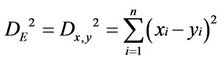 (1)
(1)
where x and y are in our case objects of dimension 24.
Recall that Pearson product-moment sample correlation coefficient “r” can be expressed as:
 (2)
(2)
where
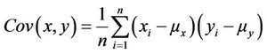
is the estimated covariance between variables x and y,  and
and  are the estimated variances of x and y, and
  and
and  are the estimates of their respective means. This statistic is widely used for summarizing the relationship between two variables or group of variables that define an object. The statistic r expresses the degree of association of two variables [21] and constitutes a standardized measure of linear dependence between them [22]. A value of r close to 1 or –1, indicates that each of the variables can be accurately predicted by a linear function of the other. The sign indicates the direction of the relationship between the Y and the X.
Two drawbacks have been traditionally accounted for the application of r [23,24]: the sensitivity of this statistic to outliers due to the fact that classical average and covariance matrices are extremely sensitive to atypical observations [25] and the inability to recognize nonlinear relationships. Outliers may play the role of inflating or deflating the r estimate since there are “good” and “bad” leverage points [25].
In order to minimize the influence of outliers we employed the MCD correlation coefficient introduced by Rousseeuw [10,26,27] that considers robust alternatives for the location and scatter estimates given in Equation (2).
MCD computes average and scatter estimates regarding a subset of h of the n data (2 < h < n) which attain the smallest determinant of the covariance matrix. Then, the location and scatter MCD estimators are given by the average and covariance matrix of the optimal subset. MCD will provide an estimate of the strength of the correlations for the data of interest free of the influence of outliers, so that a low value of the estimate would indicate that the linear relationship between the objects involved is poor. The fast-algorithm for computing MCD is complex and it is explained in detail in [28]. MCD computations have been carried out by the use of the statisticcal software package SCOUT Version 1.0 from US EPA [29]. MCD properties such as breakdown value, affine equivariance and influence function are described in [30, 31] and [32]. In order to have a wide coverage and supposed a 10% of contamination in our data, a value of h = 0.8 was chosen. Thereby the breakdown point (BDP) was about 20%, which is a value close to that recommended by [33] in order to have a balance between robustness and efficiency [25].
Distances and correlation coefficients are different approaches to measure similarity [34]. Two objects can be highly correlated (MCD ≈ 1 or –1), but their distance could be high enough to consider them as different (e.g. they could have a significantly different mean). On the other hand, the two objects can be poorly correlated (MCD ≈ 0) but DE2 could be very small and so they can both be considered as describing the same characteristics (although their differences may be due to different causes). Furthermore, according to [9] DE2 is very sensitive to additive and proportional translations while MCD is wholly insensitive to them; finally, both estimates share sensitiveness to mirror images translations. Then, for the purpose of comparing wind frequency patterns measured at two monitoring sites both correlation and proximity were considered of interest”
2.4. Assessing the Influence of the Day and the Season on Sectors 1 and 2
Wind frequencies for Sectors 1 and 2 at points A and J are considered. In order to discriminate and quantify “daily” from “seasonal” variations within the series, an “average day” was estimated by averaging hourly the corresponding hours of the day for all the data. The averaged day was later substracted to each original series. The remaining curve had still the influence of the season. The seasons through the years under study were then averaged to obtain the “average season”. The average season was later on substracted to the remaining curve (the curve resulting after the first subtraction) in order to obtain the residuals. Finally, the variances involved at the different steps of subtractions were considered in order to evaluate the degree of contribution of the “day” and the “season” to the total variation.
A trend analysis for Sectors 1 and 2 was performed as a prospective study in order to save the inexistence of simultaneous larger hourly data collections published in the area.
In both cases a nonparametric method based on local weighted regression, usually called “LOESS” or “LOW ESS” [35,36] was employed. For a sequence  the procedure computes at each given x within the range of the
 ’s a value
  as follows. Call I a window with span h around x: I = [x – h, x + h]. For
  compute weights
  where W is the “tricube” function
  for
for  and
and  otherwise. This function is maximal at x = 0 and decreases to zero at x = 1. Then for
  with
with  fit a quadratic polynomial by weighted least squares; that is, find
  such that
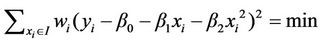
Finally put . It is usual to compute the fit at each observation, obtaining
 , but the fit can be performed at any point within the range of the
 ’s. The procedure is “nonparametric” in that the overall fitted curve
  has no explicit form and does not belong to any given parametric family. A small window span h yields a small bias but a possibly large variance, while the contrary happens with a large h; therefore h must be chosen to strike a balance between bias and variability. The nonparametric fit allows visualizing trends but it is important to discriminate whether it reveals actual data features or simply statistical artifacts. To this end the means corresponding to different time intervals were compared by estimating their standard deviations. Here it must be taken into account the lack of independence in the data. If
  is a stationary sequence with variance
  and
and  then [37]
 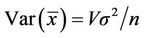 is to be computed, where V is the “inflation factor” [23]:
 ;
;  is the k-th order autocorrelation. An analysis of the data suggested that their dependence could be well represented by a first-order autoregressive process, with
  and therefore
Finally, the deviates for the mean were estimated for each window as the square root of the variance for the mean.
2.5. Exposure Corrections for Wind Velocities
An empirical approach often used in air pollutant dispersion calculations is the power law velocity profile [38,39] given by:
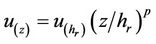 (3)
(3)
where:
 is the wind velocity “corrected” to the height z according to terrain roughness and atmospheric stability given by p;
 is the wind velocity observed at a given height;
z is the height that is desired to obtain the “corrected” wind velocity;
 is the height for the observed wind velocity.
The exponent p increases with increasing surface roughness and increasing stability. Various researches reported p values between 0.07 and 0.60. Tables given in chapter 3 of [40] were used in order to select the most appropriate value for p at points A and J. In order to avoid differences due to the effect of altitude wind velocities were corrected considering a reference height of 10 m. Besides, differences in roughness (see Section 2.2) between points A and J, were saved by affecting each point with correction factors of p = 0.25 and p = 0.15 respectively. A neutral atmospheric stability class was considered due to the fact that the seasonal averages involve day and night.
3. Results and Discussion
3.1. Sea-Land Breeze Presence
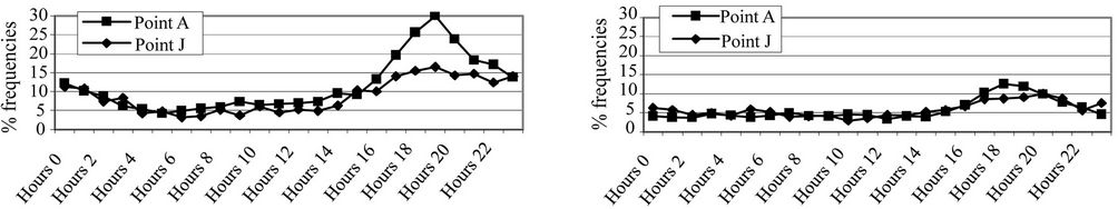
Observed wind frequencies covering the 16 directions of the compass at sites A and J for the four seasons are analyzed on hourly basis. Figure 2 shows only summer and winter patterns due to space constraints; autumn and spring displayed in most cases intermediate behaviors. Considering the lack of meteorological studies in the area the sea-land breeze phenomenon appears as the only significant source of local atmospheric variability. Its influence is more pronounced during summer due to the higher temperature contrast between the land and the large water surface of the La Plata River. For this reason summer is considered the leading season to carry out the analysis.
An overview of Figure 2 shows that wind frequencies for E (e.g. Figure 2(a1)), N (e.g. Figure 2(a13)) and NE (e.g. Figure 2(a15)) are high respect to the rest of the directions throughout the seasons in coincidence with observations carried out at La Plata Airport (Section 2.1). According to Barros et al. [41] these three wind directions, originated by the western flank of the subtropical anticyclone of the South Atlantic Ocean (located around 35˚S, 45˚W), are of major importance for the De La Plata River basin.
During the night between hours 0 and 8 the frequencies for S (Figure 2(a5)) and SSW (Figure 2(a6)) are significantly higher than those of the rest of the day. This is attributable to land-breeze because these wind directions are somewhat perpendicular to the coastline. During the first morning hours these frequencies decrease notably. As far as the influence of southern winds diminishes, wind frequencies from N (Figure 2(a13)), NNE (Figure 2(a14)) and NE (Figure 2(a15)) start to gain importance during the morning (recall that low values for NNE at Point A are due to measurement deficiencies Section 2.2). These three directions are involved with the
 (a1) E Summer (b1) E Winter
 (a2) ESE Summer (b2) ESE Winter
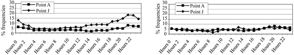 (a3) SE Summer (b3) SE Winter
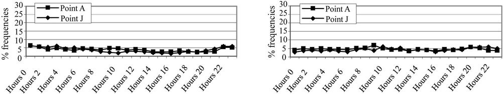 (a4) SSE Summer (b4) SSE Winter
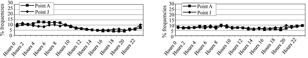 (a5) S Summer (b5) S Winter
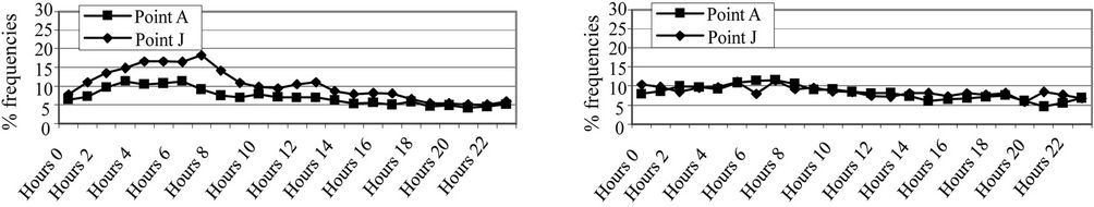 (a6) SSW Summer (b6) SSW Winter
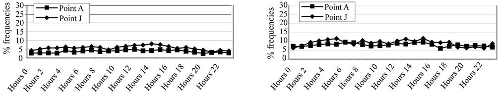 (a7) SW Summer (b7) SW Winter
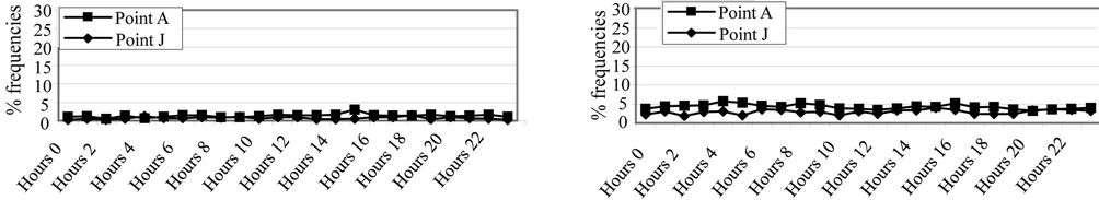 (a8) WSW Summer (b8) WSW Winter
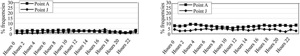 (a9) W Summer (b9) W Winter
 (a10) WNW Summer (b10) WNW Winter
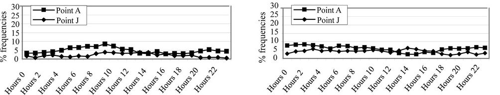 (a11) NW Summer (b11) NW Winter
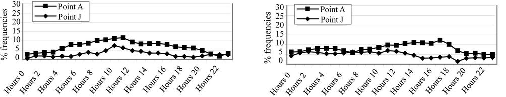 (a12) NNW Summer (b12) NNW Winter
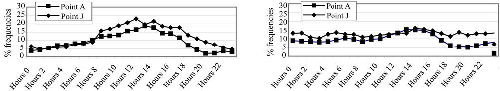 (a13) N Summer (b13) N Winter
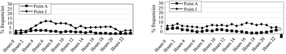 (a14) NNE Summer (b14) NNE Winter
 (a15) NE Summer (b15) NE Winter
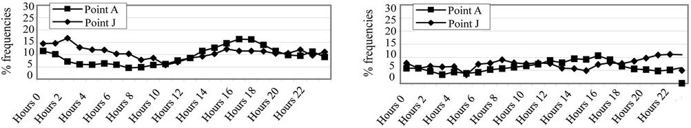 (a16) ENE Summer (b16) ENE Winter
Figure 2. Accumulated averaged frequencies (on hourly basis) of winds observed at Point A and J in summer (from (a1) to (a16)) and winter (from (b1) to (b16)) covering all the directions of the compass. Y axis indicates the percent of occurrences for a particular direction and hour respect to all the occurrences for that hour (adding all the accumulated frequencies for a given hour and season it merges 100%). X axis indicates the hour of the “day”.
first stage of the sea-breeze development that occurs during the morning hours when winds from the river start to blow towards the land. Winds flow then increasing the northerly component [42]. Sea-breeze winds follow a rotational pattern [43] clockwise, previously detected by Borque et al. [44] in a preliminary study during one day of March that revealed that the circulation rotates from NE to E between noon and dusk. This effect is observed in a second stage when N and NE winds decrease from hour 16 on (Figure 2(a13) and Figure 2(a14)) while ENE (Figure 2(a16)), E (Figure 2(a1)) and ESE (Figure 2(a2)) becomes dominant until they reach a peak during the evening (around hours 20 and 21).
Differences between points A and J for wind direction frequencies involving the land-breeze are smaller than those involving sea-breeze. A weaker land-breeze is expected mainly due to the nocturnal stability [42] but also to the city roughness that inhibits the flow of air from land to water. The wind direction spectrum observed for the land-breeze appears restricted respect to that for seabreeze. The inland penetration should be encouraged in future studies.
3.2. Similarity Analysis for Wind Direction Frequencies during the Period 1998-2003
The four seasons of the year show by inspection proximate patterns when comparing both sites (Figure 2). Warm seasons showed in general more differences between patterns than cold ones, as can be seen for summer and winter in Figure 2. This is attributable to the sealand breeze cycle that is more intense in warmer than in colder seasons [8].
Figure 2 shows major differences for NNE, NE and SE in summer while for NNE, NNW and N in winter. To analyze proximities between patterns in a more objective way the squared Euclidean distance (DE2) is employed (Table 1). This metric gives an overall estimate of the proximity between patterns but does not distinguish if the differences are concentrated in a few hours or distributed throughout the day. Therefore maximum individual differences between patterns (corresponding to one particular hour of the day) are also discussed in order to show a more complete picture of the proximity approach.
NE and NNE exhibit relative high distances throughout the seasons, often between oneand two-fold standard deviation from the mean (of DE2) (Table 1). Recalling that NNE has been deficiently measured at site A and that wind direction frequencies were expressed as a percentage for a given hour, it is possible to consider that the distortion for this direction would mainly affect the adjacent ones i.e. NE and N. Regarding these three directions the maximum individual differences throughout the day were: 12.9% in summer for NE at hour 13 (Figure 2 (a5)), 8.3% in autumn for NE at hour 12, 9.0% in winter for NNE at hour 16 (Figure 2(b14)) and 10.4 % in spring for NE at hour 11. Excluding these three directions, overall
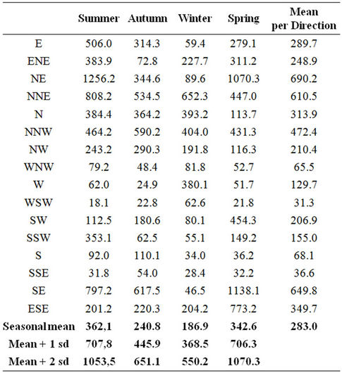
Table 1. Squared Euclidean distances covering all the directions of the compass and the four seasons.
major differences involve SE and E in summer, SE and NNW in autumn, NNW and ENE in winter and SE and SW in spring (Table 1). Except for NNE, NE and N major individual differences are 13.4% for E in summer at hour 19 (Figure 2(a1)), 10.3% in autumn for E at hour 18, 8.7% in winter for NNW at hour 17 (Figure 2(b12)), 16.4% ESE in spring at hour 20. Recalling that the group of wind directions affected by sea-breeze circulation involves NNW-ESE clockwise, most of the differences found can be attributed to this mechanism. According to Oke [45] a wind parallel with the coastline, i.e. SE, is expected to be found when the inflow of the water surface decays, but at Point A this phenomenon is not remarkably evidenced, note that during the evening SE is more important at Point J than at Point A what suggests that a more complex pattern is occurring.
Directions comprehended between SSE and NW (clockwise) are in general proximate for all the seasons (all values are below the general mean) (Table 1). This group of directions involves cold fronts, frontal waves and instability lines. Considering that the area under analysis is mainly flat, the land-breeze is weak and that the directions involved are not influenced by sea-breeze phenomenon both weather stations show proximate patterns regarding wind occurrences.
Table 2 shows the MCD estimates for the same patterns discussed above. An overview of this table shows that linear relationship between patterns are somewhat alternated

Table 2. MCD estimates between wind direction frequencies. MCD estimates tunned with h = 0.8 which implies that the subsample contain 19 of the 24 original data without contamination. In such a way the breakdown point tolerates up to 5 outliers. The average number for the outliers covering all the directions of the compass and the four monitoring sites was below 3.
with non-linear ones. Summer is the most correlated season while winter is poorly correlated. Negative MCD values, e.g. NNE in winter Figure 2(b14), indicate that predominantly, when one of the variables increases the other decreases. Note that between hours 15 and 22 the shapes of the involved curves are close to a mirror image. MCD values close to cero, e.g. ENE for winter Figure 2(b16), indicates that there is no linear relationship between the observed patterns. Throughout the seasons, there is a group of wind directions between WSW and NW (clockwise) that are poorly or negatively correlated while the group SSE-SW is highly correlated.
Taking into account both similarity criteria it emerges that wind directions between SSE and SW (clockwise) are relatively proximate and highly correlated when comparing sites through the seasons. On the other hand, NE and NNE share low proximity and poor correlations. Besides, NW is poorly correlated but quite proximate while NNW is highly correlated but the distance is relatively high.
As stated before (Section 1), short distances as well as strong linear correlations are expected to be found at two monitoring sites with common characteristics: low flat lands. Nevertheless Point A is located close to the river bank in an urban area with low buildings, while Point J is located more inland in a semi-rural area. As Ratto et al. [8] concluded, local winds are influenced mainly by sealand breeze circulations. This determines more variations in site A with respect to site J regarding some wind directions. This physical phenomenon would affect observations at both sites in a different way. The daily cycle of the sea-land breeze responds to the atmospheric pressure anomaly field induced by the cyclic thermal contrast at the surface [42]. In addition to sea-land breeze circulations as a cause of differences between sites, differences in data quality, terrain roughness and instrument exposures explain, in general, the degree of non-similarity observed at both monitoring sites.
While the distance approach generally depicts good similarity between sites as concluded in [8] the correlation approach gives an uneven picture. As evidenced by correlation analysis for some wind directions and seasons one curve for a particular wind direction can not be predicted from the other. This finding should be considered when air pollutant measurements at any site within the city need to be correlated with individual wind direction frequency observations from the point of view of sites A or J.
3.3. Influence of the Day and the Season on Sectors 1 and 2
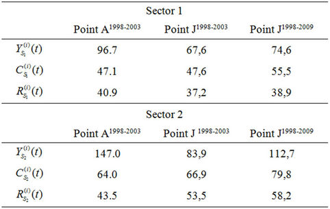
Average values for the occurrences of winds from Sectors 1 and 2 for the two periods under study are presented in Table 3. Note that considering together Sectors 1 and 2 winds transporting air pollutants from the industria sources
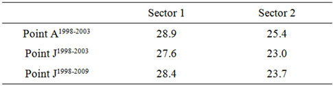
Table 3. General averages percent occurrences for Sectors 1 and 2 for the two periods under analysis.
towards exposed population (Figure 1) are occurring most of the time (above 50%). In order to gain knowledge on both sectors variations due to daily and annual cycle are considered.
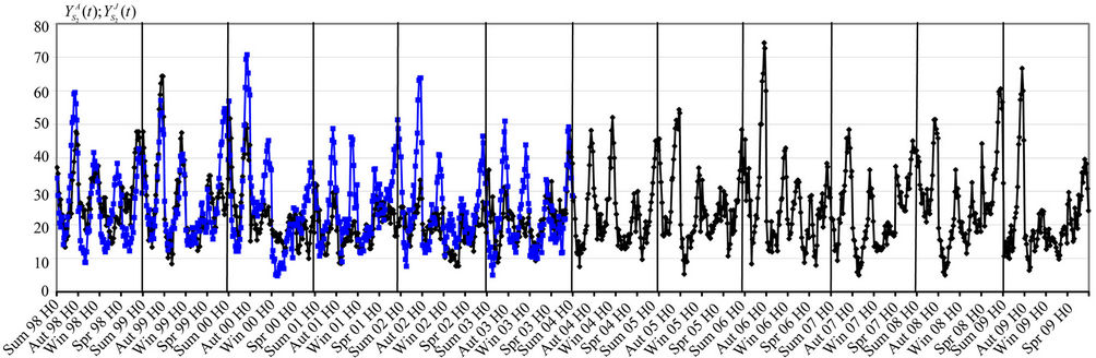
Figure 3 summarizes the analysis carried out for sector 2 during 1998-2003 (at Points A and J) and during 1998-2009 (at Point J). Due to space constraints this sector was particularly selected to show the complete steps of analysis in this section. Sector 2 is highly correlated with SO2 concentrations observed at a site downwind (Point D, see Figure 1), as was later demonstrated (see Section 3.4).
Figure 3(a) shows the evolution for the frequencies of Sector 2 from the point of view of points A  and J
and J . A particular year can be seen by visualizing its corresponding seasons in the order summer, autumn, winter and spring. There are two main contributions intended to be discriminated within the series: the influence of the “day” and the influence of the “season”. Figure 3(b) was built by averaging the days of Figure 3(a) corresponding to Points A and J for the two periods under study. From now on, and for practical purposes, the sequence of the analysis is mainly concentrated in Point A.
3.4. Series Trend
In order to detect possible remaining patterns in the series, LOESS (see Section 2.3) was applied to the residuals. The smoothed line in Figure 3(d) is the result of the application of this method to . Although no periodic pattern can be appreciated, a decreasing trend is implied at the end of the curve. To analyze features of this kind—that may appear in any of the residual graphswindows of 48 data were considered; then the mean, the first order autocorrelation coefficient and the deviation for the mean (see Section 2.3) for each window were computed (see Table 4). Since the differences between the means of consecutive windows are, in general, smaller than the deviations for the mean, there is no evidence of a significant trend for the series. Data from residuals of Sector 2 corresponding to Point J for 1998-2003 and 1998-2009 as well as the data of Sector 1 treated in the same way revealed the absence of a decreasing or an increasing trend. This result is in accordance with studies that analyze the interannual variability for the De La Plata River coast and estuary for different variables [41, 46,47].
 (a)
(a)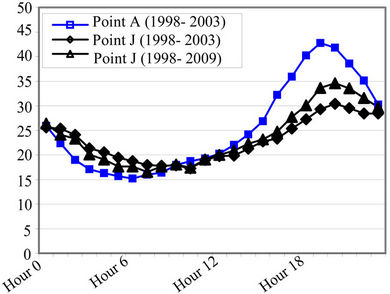 (b)
(b)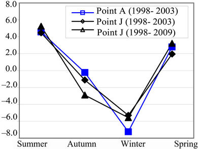 (c)
(c) (d)
(d)
Figure 3. Original serie for Sector 2, daily and seasonal influence analysis for Sector 2 from the point of view of points A (1998-2003) and J (1998-2003; 1998-2009), residuals for Sector 2 at Point A and the corresponding non parametric smoothing of the residuals. (a)  is the percent of occurrences of winds from Sector 2 respect to the occurrences for all the directions of the compass covering the period 1998-2003 (blues line).
  is analogous but for point J and covers the period 1998-2009 (black line); for analysis purposes this series is divided into two periods 1998-2003 and 1998-2009. Each individual point represents the frequency of winds from sector 2 (taken from the corresponding wind rose) for a given hour (t) and for a particular season and year. Values for t are identified each 24 data and are expressed in an abbreviated way, e.g. Sum 00 H0 represents the frequency for Hour 0 of summer 2000 corresponding to Sector 2. The whole data set has 576 points for Point A (covering six years) while 1152 points for Point J (covering 12 years); (b) The Y axis represents the percent of occurrences for the average day for Sector 2 from the point of view of points A (blues line) and J for the two periods under study (black line). It was built by averaging each accumulated hour through all seasons and years; (c) The Y axis represents the percent of occurrences for the average for the seasons; (d) Residuals for the series of (a) at Point A. The smoothed line was obtained by the application of the locally weighted regression method. Vertical lines indicate the starting of the year.

Table 4. Series trend. Mean, first order autocorrelation coefficient and deviate for the mean for each window of 48 data covering the 576 data for the residuals for Sector 2 at Point A.
By subtracting the averaged day observed at Point A (Figure 3(b)) to the original series  (Figure 3(a)) the resulting curve
  (not shown) is expected not to have this influence.
  has still the influence of the seasons. When averaging them values of 3.44 for summer, –2.96 for autumn, –1.57 for winter and 1.09 for spring were obtained (see Figure 3(c)). By subtracting seasonal values to
  the remaining curve (residuals for Sector 2 at Point A, i.e.
 ) will have neither the influence of the day nor that of the season (see the cloud points in Figure 3(d)).
Following the same procedure the residuals for Point J for the period 1998-2003 and for the period 1998-2009 were obtained. The same protocol (not shown due to space constraints) was carried out to Sector 1 data (Figure 4). To measure the variation removed by each of the two subtracting steps the variances were computed (see Table 5(a)). For example, subtracting the variance of the remaining series  from the variance of the original
  a value of 83 (147.0 - 64.0) is obtained. This means that 56.5% of the original variance corresponds to the influence of the day (see influence of the day (IOD) for Sector 2 in Table 5(b)). The difference in variances between
  and
and  is 20.5 and represents only 13.9% (the percent of variance caused by the influence of the season) of the total variation (see influence of the season (IOS) for Sector 2 in Table 5(b)). Finally, the variance of the residuals represents 29.6% of the original variance and constitutes the unexplained fraction of the total variance (see unexplained variance (UNE) for Sector 2 in Table 5(b)). An overview of Table 5(b) shows that Point A has more variation due to the day than Point J and this variation is slightly more pronounced for Sec-
 (a)
(a) (b)
(b)
Table 5. Variances and percent of variances. (a) Variance for the original series, variance for the remaining series after the subtraction of the influence of the day and variance for the residuals according to the procedure explained in Section 2.4 (i) corresponds to the sector and period of the corresponding headings of the columns. (b) % of variation attributed to the influence of the day, the season and unexplained respect to the total variance of the original series. a% of variance attributable to the influence of the day; b% of variance attributable to the influence of the season; c% of unexplained variance.
tor 2 than for Sector 1. These results imply that Sector 2 at site A (more close to the river) receives more contribution from the sea-breeze circulation and its rotation along the day than Sector 1. Winds from Sector 1 are mainly originated by the South Atlantic subtropical anticyclone and in part from the morning sea-breeze. As both sites have differences mainly due to terrain roughness the influence of the anticyclone may be considered the same for both sites. Point J is more inland and therefore receives less influence from the sea-breeze. So, independently from the season, Point A receives more influence from the sea-breeze during the day than Point J (this can be appreciated comparing absolute values for the variances at sites A and J for the original series in Table 5(a)). As the gap between IOD and IOS at site J is smaller (than at site A) the annual cycle appears more visible at Point J.
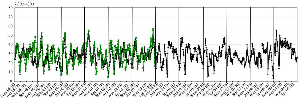
Figure 4. Analogous to Figure 3(a) this figure represent the original series for Sector 1 from the point of view of points A covering 1998-2003 (green line) and J covering 1998-2009 (black line).
3.5. Wind Direction Frequencies and Air Pollutants
Figure 5 shows hourly occurrences for Sector 2 involving spring 2005 at site J, the spring average for the period 1998-2003 at site J, the spring average for the period 1998-2003 at site A and SO2 concentrations (ppbv) observed during spring 2005 at Point D [12]. The low values observed for SO2 were attributed to the distance between industrial sources and the site the monitoring device was allocated. SO2 concentrations are represented in a different scale in order to better visualize its hourly variation and further compare its shape with different cases of Sector 2.
The high MCD values obtained (Table 6) show an example of how observed averaged industrial pollutants detected at site D may depend linearly on winds from Sector 2.
An MCD estimate correlating the average of Sector 2 at Point A and the average of Sector 2 at Point J during 1998-2003 gives 0.795, a relatively high value when compared individually to the wind directions composing the sector (i.e. ENE, E and ESE) (Table 2). The same occurs when correlating averages for Sector 1 for the same period (MCD is 0.953). This behavior allows correlating air pollutant measurements carried out wherever within the city area with Sectors 1 and 2. Note that this is not possible when individual wind direction frequencies are involved (Section 3.2).
3.6. Wind Velocities and Calms
In order to provide context for the wind direction frequency analysis we summarized information regarding averaged wind velocities and calms. Table 7 shows observed wind velocities at points A and J for both periods under study and their corresponding corrected values estimated with Equation (3). Observed values at Point A are higher than those observed at Point J; within the boundary layer friction forces decrease with height. With the application of Equation (3) differences between sites tend to be negligible.
Although meteorological observations carried out at airports are not very appropriate for air pollution considerations [48] we took into account La Plata Airports’ monthly
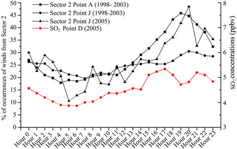
Figure 5. Left Y axis refers to the % occurrences of winds from Sector 2 (on hourly basis-X axis) observed at Point A and J for spring for different periods. Right Y axis refers to SO2 concentration hourly averages observed during a short monitoring campaign at Point D during spring 2005.
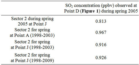
Table 6. MCD values obtained when correlating observed hourly SO2 concentrations and wind frequencies from Sector 2 for different sites and time scales.
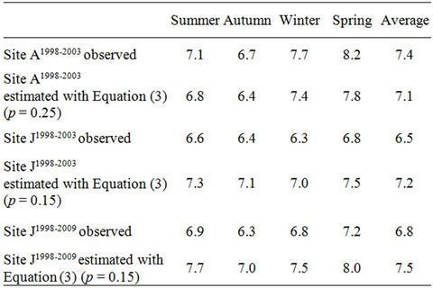
Table 7. Averaged wind velocities (km·h–1) observed at points A (12 m height) and J (5 m height) and their corresponding corrected values according to Equation (3) (Section 2.5).
data during the decade 2001-2010 [20] available from the National Meteorological Service to provide context for our measurements. Averaged velocities for 8 direction wind roses at the Airport located in a plain open area measured at 10 m above the ground were: 14.7 km·h–1 in summer, 12.7 km·h–1 in autumn, 13.4 km·h–1 in winter, 15.0 km·h–1 in spring (Figure 1). These values are around 2 times higher than those at points A and J corrected to 10 m height. This difference can be attributed to differences between urban and rural climates [49] and in terrain roughness [50]. An average wind velocity of 13.0 km/h covering the period 1967-1994 measured at a height of 40 m at the Observatory of the National University of La Plata located 1 km far south from Point A supports this idea [51].
Averaged calms at points A and J for both periods under study are shown in Figure 6; on average observed calms at point A are around half of those corresponding to point J. This can be explained in terms of differences in height of the anemometers (within the boundary layer friction forces decrease with height) but also due to data quality differences (see Section 2.2). Calms at the airport follow a similar trend that those of Point J.
4. Conclusions
The hourly analysis of winds observed at the two sites allowed detect the presence of local sea-land breeze circulations in the context of synoptic scale winds. Seabreeze develops from N to ESE (clockwise) during the daytime while land-breeze takes place following a weaker pattern involving S and SW winds.
The two methods employed to assess similarity between sites allowed to gain insight of wind patterns. The distance approach showed in general good similarities. On the other hand, the robust correlation approach revealed the absence of a generalized linear correlation
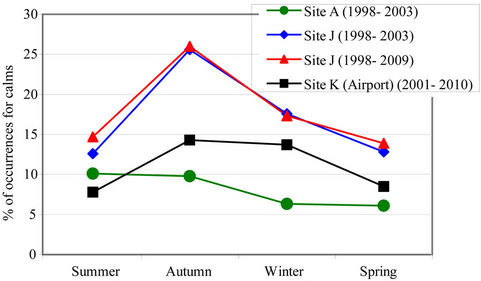
Figure 6. Calm occurrences observed at different sites of the city and surroundings.
between patterns at both sites. This issue should be taken into account when correlations between air pollutant concentrations and individual wind direction frequencies need to be considered. Detected differences in hourly wind direction patterns between sites are mainly attributable to the sea-land breeze phenomenon but also differences in terrain roughness, data quality and instrument exposures are to be taken into account.
The analysis of series corresponding to Sectors 1 and 2 allows a preliminary assessment of the probability of occurrences and the characterization of the daily and annual cycles of both sectors. General mean for Sectors 1 and 2 observed at both sites are very similar. Winds from any of the two sectors may occur more than 50% of the time which is very important considering the transport of air pollutants towards exposed population. The influence of the day was found to be more pronounced than the influence of the season for both sectors and sites, but at Point A (close to the river bank) the gap is more important due to the sea-land breeze effect.
The trend analysis employing LOESS with the further computing of the mean and deviate from the mean for different time intervals proved to be a sound approach. The analysis of the residuals for Sectors 1 and 2 series showed there was no remaining pattern when subtracting the effect of the day and the season.
Correlations between wind direction frequency averages for Sector 1 and 2 at both points A and J are strong. This implies that air pollutants measured at any site within La Plata area can be correlated with winds from Sectors 1 and/or 2 observed at sites A or J. The robust correlation coefficient revealed, as an example, the linear character of dependence between winds from Sector 2 and sulfur dioxide concentrations.
Observed and corrected wind velocities showed a general agreement when comparing sites. Wind velocities observed at the airport (reference) were found to be around two times higher than those observed at sites A and J. This difference can be attributed to differences between urban and rural climates but also in data quality and terrain roughness. Differences in calms between sites are attributed to differences in instrument exposure, data quality and roughness.
5. Acknowledgements
The authors are grateful to UTN-National Technological University (Regional Faculty at La Plata) for the equipment and facilities supplied regarding the monitoring site “Point A” and to Dr. Christian Weber for the data regarding “Point J”. Our particular thanks to Lic. Nelly Cap and Dr. Gustavo Torchia from CIOp for their contributions to this paper. Feder Funds and Fundación Parque y Científico de Albacete provided the hiring of Andrés Nico
REFERENCES
- N. A. Mazzeo, L. E. Venegas and H. Choren, “Analysis of NO, NO2, O3 and NOx Concentrations Measured at a Green Area of Buenos Aires City during Wintertime,” Atmospheric Environment, Vol. 39, No. 17, 2005, pp. 3055-3068. doi:10.1016/j.atmosenv.2005.01.029
- M. I. Glassmann and N. A. Mazzeo, “Air Pollution Potential: Regional Study in Argentina,” Environmental Management, Vol. 25, No. 4, 2000, pp. 375-382. doi:10.1007/s002679910029
- C. Bilos, J. C. Colombo, C. N. Skorupa and M. J. R. Presa, “Sources, Distribution and Variability of Airborne Trace Metals in La Plata City Area, Argentina,” Environmental Pollution, Vol. 111, No. 1, 2001, pp. 149-158. doi:10.1016/S0269-7491(99)00328-0
- L. Massolo, A., Müller, M., Tueros, M., Rehwagen, U. Frank, A. Ronco and O. Herbarth, “Assessment of Mutagenicity and Toxicity of Different-Size Fractions of Air Articulates from La Plata, Argentina, and Leipzig, Germany,” Environmental Toxicology, Vol. 17, 2002, pp. 219-231. doi:10.1002/tox.10054
- L. Massolo, A. Müller, O. Herbarth, A. Ronco and A Porta, “Air Pollution and Children’s Health in Urban and Industrial Areas of La Plata, Argentina,” Acta Bioquímica Clínica Latinoamericana, Vol. 42, No. 4, 2008, pp. 567- 574.
- D. S. Nitiu, “Aeropalynologic Analysis of La Plata City (Argentina) during 3-Year Period,” Aerobiologia, Vol. 22, 2006, pp. 79-87. doi:10.1007/s10453-005-9009-4
- M. M. Negrin, M. T. Del Panno and A. E. Ronco, “Study of Bioareosols and Site Influence in the La Plata Area (Argentina) Using Conventional and DNA (Fingerprint) Based Methods,” Aerobiologia, Vol. 23, No. 4, 2007, pp. 249-258. doi:10.1007/s10453-007-9069-8
- G. Ratto, R. Maronna and G. Berri, “Analysis of Wind Roses Using Hierarchical Cluster and Multidimensional Scaling Analysis at La Plata, Argentina,” Boundary Layer Meteorology, Vol. 137, No. 3, 2010, pp. 477-492. doi:10.1007/s10546-010-9539-3
- C. Romesburg, “Cluster Analysis for Researchers,” Lulu Press, Raleigh, 2004.
- P. J. Rousseeuw, “Multivariate Estimation with High Breakdown Point,” In: W. Grossmann, G. Pflug, I. Vincze and W. Wertz, Eds., Mathematical Statistics and Applications, Reidel, Dordrecht, 1985, pp. 283-297. doi:10.1007/978-94-009-5438-0_20
- A. D. Gordon, “Classification,” 2nd Edition, Chapman and Hall/CRC, Boca Raton, 1999.
- ] G. Ratto, F. Videla and R. Maronna, “Analyzing SO2 Concentrations and Wind Directions during a Short Monitoring Campaign at a Site Far from the Industrial Pole of La Plata, Argentina,” Environmental Monitoring and Assessment, Vol. 149, No. 1-4, 2009, pp. 229-240. doi:10.1007/s10661-008-0197-6
- Y. Qian, K. Migliaccio, Y. Wan and Y. Li, “Trend Analysis of Nutrient Concentrations and Loads in Selected Canals of the Southern Indian River Lagoon, Florida Trend Analysis of Surface Water Nutrients,” Water Air and Soil Pollution, Vol. 186, No. 1-4, 2007, pp. 195-208. doi:10.1007/s11270-007-9477-y
- X. Fan, B. Gu, E. Hanlon, Y. Li, K. Migliaccio and T. Dreschel, “Investigation of Long-Term Trends in Selected Physical and Chemical Parameters of Inflows to Everglades National Park 1977-2005,” Environmental Monitoring Assessment, Vol. 178, No. 1-4, 2011, pp. 525-536. doi:10.1007/s10661-010-1710-2
- G. Ratto, F. Videla, J. R. Almandos, R. Maronna and D. Schinca, “Study of Meteorological Aspects and Urban Concentration of SO2 in Atmospheric Environment of La Plata, Argentina,” Environmental Monitoring and Assessment, Vol. 121, No. 1-3, 2006, pp. 327-342. doi:10.1007/s10661-005-9127-z
- C. W. Thornthwaite, “An Approach toward a Rational Classification of Climate,” Geographical Review, Vol. 38, No. 1, 1948, pp. 55-94. doi:10.2307/210739
- J. C. Gianibelli, J. Köhn and E. E. Kruse, “The Precipitations Series in La Plata, Argentina and Its Possible Relationship with Geomagnetic Activity,” Geofísica International, Vol. 40, No. 4, 2001, pp. 309-314.
- SMN, “Estadísticas Climatológicas. Servicio Meteorológico Nacional 1981-1990,” Serie B, No. 37. SMN, Buenos Aires, 1992.
- SMN, “Estadísticas Climatológicas. Servicio Meteorológico Nacional 1991-2000,” SMN, Buenos Aires, 2000.
- SMN, “Estadísticas Climatológicas. Servicio Meteorológico Nacional 2001-2010,” SMN, Buenos Aires, 2011.
- V. Conrad and L. W. Pollak, “Methods in Climatology,” Harvard University Press, Cambridge, 1950.
- C. Cuadras, “Métodos de Análisis Multivariante,” EUB S.L., Barcelona, 1996.
- D. S. Wilks, “Statistical Methods in the Atmospheric Sciences,” 2nd Edition, Elsevier, New York, 2006.
- S. Chatterjee and A. S. Hadi, “Regression Analysis by Example,” 4th Edition, John Wiley and Sons, Hoboken, 2006. doi:10.1002/0470055464
- C. Croux and G. Haesbroeck, “Influence Function and Efficienty of the Minimum Covariance Determinant Scatter Matrix Estimator,” Journal of Multivariate Analysis, Vol. 71, No. 2, 1999, pp. 161-190. doi:10.1006/jmva.1999.1839
- P. J. Rousseeuw and A. M. Leroy, “Robust Regression and Outlier Detection,” John Wiley and Sons, New York, 1987. doi:10.1002/0471725382
- P. J. Rousseeuw, “Least Median of Squares Regression,” Journal of the American Statistical Association, Vol. 79, 1984, pp. 871-880. doi:10.2307/2288718
- P. J. Rousseeuw and K. Van Driessen, “A Fast Algorithm for the Minimum Covariance Determinant Estimator,” Technometrics, Vol. 41, No. 3, 1999, pp. 212-223. doi:10.2307/1270566
- US EPA, “Scout 2008 Version 1.0 User Guide Second Edition,” EPA/600/R-08/038, 2009. http://www.epa.gov/esd/databases/scout/abstract. htm#Scout2008v101
- R. A. Maronna, R. D. Martin and V. J. Yohai. “Robust Statistics. Theory and Methods,” John Wiley and Sons Ltd., West Sussex, 2006. doi:10.1002/0470010940
- M. Hubert and M. Debruyne, “Minimum Covariance Determinant,” Computational Statistics, Vol. 2, No. 1, 2010, pp. 36-43.
- M. Hubert, P. J. Rousseeuw and T. Verdonck, “A Deterministic Algorithm for the MCD,” Technical Report TR-10-01, Department of Mathematics Katholieke, Universiteit Leuven, Leuven, 2010.
- C. Fauconnier and G. Haesbroeck, “Outliers Detection with the Minimum Covariance Determinant Estimator in Practice,” Statistical Methodology, Vol. 6, No. 4, 2009, pp. 363-379. doi:10.1016/j.stamet.2008.12.005
- L. F. Escudero, “Reconocimiento de Patrones,” Paraninfo, Madrid, 1977.
- W. S. Cleveland, “Robust Locally Weighted Regression and Smoothing Scatterplots,” Journal of the American Statistical Association, Vol. 74, No. 368, 1979, pp. 829- 836. doi:10.2307/2286407
- W. S. Cleveland and S. J. Devlin, “Locally Weighted Regression: An Approach to Regression Analysis by Local Fitting,” Journal of the American Statistical Association, Vol. 83, No. 403, 1988, pp. 596-610. doi:10.2307/2289282
- G. Box, G. M. Jenkins and G. Reinsel, “Time Series Analysis: Forecasting & Control,” 3rd Edition, Wiley, New York, 2008.
- S. P. Arya, “Introduction to Micrometeorology,” 2nd Edition, Academic Press, San Diego, 2001.
- J. H. Seinfeld and S. N. Pandis, “Atmospheric Chemistry and Physics. From Air Pollution to Climate Change,” 2nd Edition, John Wiley & Sons, Hoboken, 2006.
- K. Wark, C. Warner and W. Davis, “Air Pollution. Its Origin and Control,” 3rd Edition, Addison Wesley Longman, Berkeley, 1998.
- V. Barros, A. Menéndez and G. Nagy, “El Cambio Climático en el Río de la Plata,” CIMA, Buenos Aires, 2005.
- G. J. Berri, L. Sraibman, R. Tanco and G. Bertossa, “Low-Level Wind Field Climatology over the La Plata River Region Obtained with a Mesoscale Atmospheric Boundary Layer Model Forced with Local Weather Observations,” Journal of Applied Meteorology and Climatology, Vol. 49, No. 6, 2010, pp. 1293-1305. doi:10.1175/2010JAMC2370.1
- J. E. Simpson, “Sea Breeze and Local Wind,” Cambridge University Press, Cambridge, 2006.
- P. Borque, J. Ruiz, Y. G. Skabar, L. Aldeco, A. Godoy and M. Nicolini, “Numeric Simulation of a Real Sea Breeze Event in La Plata River,” XV Congreso Brasileño de Meteorología, CBMET XV, San Pablo, August 2008.
- T. R. Oke, “Boundary Layer Climates,” 2nd Edition, Routledge, London, 1987.
- W. Dragani, P. Martin, C. Simionato and M. Campos, “Are Wind Wave Heights Increasing in South-Eastern South American Continental Shelf between 32°S and 40°S?” Continental Shelf Research, Vol. 30, No. 5, 2010, pp. 481-490. doi:10.1016/j.csr.2010.01.002
- G. Escobar, I. Camilloni and V. Barros, “Desplazamiento del Anticiclón Subtropical del Atlántico Sur y su Relación con el Cambio de Vientos Sobre el Estuario del Río de la Plata,” X Congreso Latinoamericano e Ibérico de Meteorología (CLIMET) y II Congreso Cubano de Meteorología, SOMETCUBA y FLISMET, La Habana, March 2003,.
- G. C. Holzworth, “Mixing Depths, Wind Speeds and Air Pollution Potential for Selected Locations in the United States,” Journal of Applied Meteorology, Vol. 6, No. 6, 1967, pp. 1039-1044. doi:10.1175/1520-0450(1967)006<1039:MDWSAA>2.0.CO;2
- H. E. Landsberg, “The Urban Climate,” Academic Press, New York, 1981.
- M. I. Glassmann, C. F. Pérez and J. M. Gardiol, “SeaLand Breeze in a Coastal City and Its Effect on Pollen Transport,” International Journal of Biometeorology, Vol. 46, No. 3, 2002, pp. 118-125. doi:10.1007/s00484-002-0135-1
- G. Ratto, F. Videla, R. Maronna, A. Flores and F. De Pablo, “Air Pollutant Transport Analysis Based on Hourly Winds in the City of La Plata and Surroundings, Argentina,” Water Air and Soil Pollution, Vol. 208, No. 1-4, 2010, pp. 243-257. doi:10.1007/s11270-009-0163-0
NOTES
*Corresponding author.