International Journal of Astronomy and Astrophysics
Vol.04 No.04(2014), Article ID:52409,20 pages
10.4236/ijaa.2014.44058
Determining Attitude and Position in Deep Space Missions Using X Ray Pulsars
Amir Moghtadaei Rad1*, Leila Vahid Azari2
1Electrical Engineering Department, Hashtgerd Branch of Islamic Azad University, Alborz, Iran
2Science Department, Hashtgerd Branch of Islamic Azad University, Alborz, Iran
Email: *amir.moghtadaei@hiau.ac.ir
Academic Editor: Ran Zhou, Fermi National Accelerator Laboratory, USA
Copyright © 2014 by authors and Scientific Research Publishing Inc.
This work is licensed under the Creative Commons Attribution International License (CC BY).
http://creativecommons.org/licenses/by/4.0/


Received 22 September 2014; revised 20 October 2014; accepted 15 November 2014
ABSTRACT
This paper initially reviews types of deep space navigation methods. Then, it studies the use of pulsars as one of sources emitting electromagnetic waves in navigation; hence more details regarding the pulsar physics and the history of navigation using pulsars are presented. The various methods of navigation (including radio method), their advantages and disadvantages―in comparison with navigation using pulsars in spacecraft―are discussed. Then, the equations necessary for calculating position and velocity of a spacecraft (such as the arrival time of pulse from pulsar to the receiver) are introduced, and the methods of calculating position and velocity are dealt with. Finally, two algorithms are presented for positioning, and one for velocity. Attitude determination follows the same simple methods presented in various articles.
Keywords:
Pulsar, Neutron Star, Attitude Determination, Positioning, Spacecraft

1. Introduction
Deep space navigation has its own circumstances and differs considerably from the usual methods of navigation on earth or around it. There are various methods of spacecraft navigation.
1) Orbit Determination: This is the process by which the dynamics of a vehicle turning in a certain orbit are determined. It is employed in order to determine and control the position of satellite or spacecraft by earth stations.
2) Orbit Propagation: This is the process by which the dynamics of an orbiting vehicle by using the model of functioning forces on it are transited into the orbit around which it is turning. Determining these dynamics, analytically or numerically, would lead to the estimation of the best state of the flying object regarding velocity or position.
3) Orbit Navigation: The process of determining position, velocity, attitude, angle velocity using external sensors, surely in combination with some internal information, is called orbit navigation.
The 3-dimensional position of the majority of spacecraft and satellites moving in specified orbits around celestial bodies is obtainable employing much more simple methods as well. However, it is difficult in some cases to control their path, and unmodelled and unpredictable disturbances. This would lead to the deviation of the flying object from its major path. Hence, orbit determination methods with the help of earth stations, and by using sensors inside the spacecraft can improve this. Radar methods and optical tracing are important methods in determining orbits of satellites. In radar methods, the position of the spacecraft in relation to the earth stations is calculated through the signals transmitted to and received from the satellite. In spite of the precision the methods might possess in one direction, they do not have the required precision in two directions. As an example, precision in Viking Mars measurer was 50 kilometers in the major direction while it was several hundreds of kilometers in two directions. However, several measurements of position over time by radars can lead to the desired precision.
Moreover, it is necessary in these methods to have the exact position of antennae and earth stations for exactly determining the position of spacecraft; as the spacecraft goes away from the earth, positioning error increases due to the infeasibility of exact estimation of the position of earth stations.
Although radar methods based on earth stations do not need any complicated hardware to be installed in spacecraft, there will be need for complicated calculations and analyses in earth processors.
Deep Space Network, one of these radar networks for spacecraft positioning, consists of three earth stations located an angle of 120 in three spots of earth namely California in USA, Madrid in Spain, and Canberra in Australia. Despite employing interferometry techniques through the calculation of several signals of difference received from different stations, there are again changes in positioning as the spacecraft gets away from the earth. The utmost precision achievable through this network and the VLBI technique would be 1 to 10 kilometers in astronomical unit. Optical tracing method is very much similar to radar methods; the difference is that it navigates relying on receiving returned visible light from the spacecraft. In other words, photos or films are taken using stars or planets. Then comparing the parameters of celestial bodies in the photos or films with the parameters of stars or planets neighboring the celestial bodies, the relative position of the spacecraft in relation to the intended planet is calculated. It should be mentioned that having known the position of an intended planet in relation to space, the absolute position of the spacecraft is also determinable, though the calculation of relative position would suffice in discovery missions. The method relies heavily on the atmosphere of planets, and the environmental factors, which is itself a separate matter. Moreover, the method is very costly. The need to be close to the intended planet for the sake of photography is another disadvantage of the method. The exact positioning of aircraft requires a blend of both radar and optical methods after all.
Moreover, having the exact time in navigation in order for the spacecraft to communicate with earth stations, and to determine the position of other planets is of great significance. The time is measured and updated by atomic clocks. For instance, tracing a radio signal with an error of several meters having been transmitted from an earth station requires the time with a precision of nano seconds in several hours.
The attitude of the spacecraft, as mentioned in many earlier researches, is calculated by gyroscopes in inertial frames, and with magnetic, solar, and astronomical sensors in relation to earth. What is emphasized more in this and other similar papers, however, is determining position, velocity, and time in Deep space and inter-planet missions.
Next, various methods of determining time, position and attitude, and comparisons of them are presented (Table 1):
The discoveries in the field of solar system having increased, scientists have become more interested in employing earlier, less expensive, and more exact methods. Independent navigation by the spacecraft itself and with no interference on the part of the earth station equipment is one consequence of discoveries in the last 50 years. The use of sources transmitting electromagnetic waves (in various wave lengths) is one of the first methods employed in independent spacecraft navigation. Hence, pulsars, as one of sources transmitting electromagnetic waves, are next introduced.
2. Variable Celestial Sources
Celestial bodies have been great aids in navigation for passengers and flying objects throughout history. Of course,

Table 1. Comparison of advantage and disadvantage of different navigation method in spacecraft [1] .
the majority of these bodies had a fixed, stable radiation and was known as stable stars in the space. Recently, some sources that produce variable very intense electromagnetic waves with various wave lengths have been identified the variation of which reaches the earth or spacecraft periodically or non-periodically (known as variable celestial sources). The name is due to the variability of the intensity of the radiation emitted from them. These individual stars have a uniquely identifiable, periodic, and predictable signal; so they can be utilized for navigation purposes. One of the variable celestial sources used frequently in spacecraft navigation is the pulsars. A pulsar is a neutron star rotating very rapidly, and visible as a pulsate source of electromagnetic radiation. Neutron stars are formed when a class of stars collapse, and from conservation of angular momentum, as the star becomes smaller, or more compact, they rotate faster. The conservation of magnetic flux forms a magnetic field at the surface of the star, up to 1023 gauss/cm3 or more. The resultant body is both a rotating heavy surface and a strong accelerator of particles since a rotating magnetic field forms strong electrical fields accelerating charged particles. The accelerated particles emit electromagnetic waves in all spectra―from radio waves to Gama―which are very much likely to radiate in the direction of magnetic axes. If the magnetic axis is not in the same direction as the rotating axis (which is usually the case as in the earth), a faraway beholder will observe a pulse of radiation when the pulse inclined towards the magnetic axis is in the direction of the line-of-sight. This is exactly similar to the visible light from the lighthouse, the power of which is actually the rotating power saved in the neutron star. As the energy is emitted slowly, the rotating velocity of the star decreases along with longer periods. These sources are hence called rotation-powered pulsars.
The sources will radiate with a time epoch of 10 million years. Then their rotation velocity will decrease with a period of 10 seconds, and will no longer be able to produce the required strong field for accelerating particles that emit powerful radiation.
Pulsars the period of which changes nearly 100 ns per year have proven to be very exact clocks throughout their lifetime. However, even this little velocity reduction leads to disequilibrium, and gradual and sudden disorder in the state of the star. These unpredictable disorders limit the utilization of the ordinary pulsars as navigation control towers.
There are nearly 100,000 celestial sources 38,500 of which lie in the visible range. The first variable celestial source was discovered by Tycho and Schuler in 1572 in Cassiopeia constellation [2] . The second was a 1 micron star discovered in crocodile constellation by Fabricius [3] in 1596.
Variable celestial sources are divided into sources with regular and irregular periods. Due to the feasibility of measurement of their period phase, sources with regular periods (of which pulsars are one type) are utilized in navigation. Another reason for the utilization of variable sources, instead of constant sources (like stars) in navigation is that the constant signals emitted from millions of stars show more chance of error and deviation than the signals produced with a single period. This is exactly like optical signals produced by the lighthouse in marine navigation. The light gets to the receiver with a certain period. It is this period which avoids from the sight error of a constant signal.
3. The History of Pulsar-Based Navigation
Pulsars were first discovered in radio spectrum by Bell and Hewish in 1967 [4] - [6] . Richly, Downs, and Morris [7] - [10] , proposed the use of pulsars (as exact clocks for earth systems) in 1971. Employing the facilities of Deep Space Network available for NASA, Richley and Downs [11] , managed to measure the TOA of pulses of pulsars in 1980. Employing pulsars as exact atomic clocks was confirmed by articles and researches by Allan, Matsakis, Taylor [12] [13] , in the 1980s and 1990s. This led to the introduction of pulsars as exact clocks in navigation.
In 1974, a method of space navigation employing radio pulsars was proposed by Downs [14] . The method was based on installing 3-9 pyramidal antennae (of two meters of length) on all sides of the spacecraft in order to scan all the 3-dimensional space around the spacecraft for receiving radio signals emitted by pulsars. It was possible to estimate the position of the spacecraft with a precision of 150 km in this way.
Radio and optical pulsars both have disadvantages which makes it impossible to use them extensively in navigation.
The disadvantages of both radio and optical pulsars render their extensive utilization impossible in navigation. Faintness and underexposure of radio signals required the use of large antennae in order to compensate for this deficit. Another disadvantage of the method was the long time required for signal absorption in order to reduce the proportion of noise to signal. In the case of optical signals, due to the pulsars in this electromagnetic spectrum being few and faint, very strong and large telescopes were needed to absorb their futons. Moreover, luminous planets neighboring these pulsars strongly increased the possibility of presence of noise in the light received from optical pulsars.
Scientists were, thus, interested in X-spectrum electromagnetic pulsars in the 1970s―waves with the frequency of 1 - 20 Kev . In 1981, Chester and Butman propounded utilization of X-ray pulsars for satellite navigation around the earth [15] . They proposed 17 pulsars with desired convergence in X ray―which were recoverable by using a detector with a diameter less than 0.1 m compared to the antennae used for absorbing radio waves, and the telescopes used for absorbing optical waves, the detector was much less bulky. Comparing the TOA of pulsar signals to the satellites in the earth orbit with far away space craft, they were able to estimate the position of spacecraft in a 24-hour cycle with a precision of 150 km.
In 1993, Wood put forth a method for determining attitude, position, and time of satellite ARGOS under the project of NRL-801 [16] . In addition to X pulsars, celestial sources with persistent radiation were also used in navigation especially in determining positioning and attitude. Actually the star tracker was used for attitude determination, the horizontal surface of the earth or moon for positioning, and X-ray pulsars for the exact determination of time.
In 1996, Hanson used a 2-dimensional detector for determining attitude, and X-ray pulsars for determining time. His proposal was applied in the spacecraft HEAD-1 and the attitude was determined with a precision of 01 - 0.01 degrees [17] .
Since 1999 and 2000, various methods of using X-ray pulsars especially in spacecraft positioning were employed in different projects namely ARGOS [18] [19] .
Pulsar Physics
Changes of signal intensity in variable celestial sources are either intrinsic or extrinsic. Intrinsic variable sources are divided into pulsating and eruptive. Through the expansion or contraction of their limb, pulsating variable sources emit electromagnetic waves radically or non-radically. In eruptive variable sources, on the other hand, electromagnetic waves are produced by intense nuclear eruption, and transmission of energy from the nucleus to the surface of the star.
Extrinsic variable celestial sources are divided into rotating star, Eclipsing Binaries, and Cataclysmic variables.
Rotating stars turn very rapidly around their axes. The rotation accelerates the charged particles inside the stars, which radiate in electromagnetic waves of different spectra (Figure 1).
Binaries are the pair stars turning round the center of their common body. The bright star is known as the main star, and the less bright one is known as the companion star.
The Eclipsing kind is the one in which the rotation plate of the stars is located in the direction of the eye-sight of the viewer in a way that one star hides alternately along its path behind the other. It seems to the viewer as if the light of the star decreases and increases (Figure 2).
When the system of binaries includes one very dense body, like the White Dwarf, the neutron star or the black

Figure 1. Layers of a neutron star [20] .

Figure 2. Representation of eclipsing binaries [20] .
hale along with another star, the gases on the surface of the second star are absorbed by the first during magnetic storms along which a lot of gravity potential is released. The release of the potential would emit electromagnetic energy. If the gases are absorbed by the White Dwarf, Cataclysmic variables are formed. On the other hand, if the gases are absorbed by the neutron star or the black Hale, the stars would be called the X-spectrum binaries (Figure 3).
4. Utilizable Stars in Navigation
Stars with relatively much light or energy, durability, stable period, and little pulse width are utilizable in spacecraft navigation. They are used in navigation because of no need for huge detectors, their simplicity, and rapid recognition. Due to the unpredictability of their period, and their unstable and endurable behavior, Eruptive and Cataclysmic stars are thus of not much use in signal transmission in navigation.
Rotating stars and Eclipsing Binaries, on the other hand, are extensively utilized in navigation because of permanence of their signal, and their stable period of signal transmission. There is, however, need for a good deal of compensation at the time of detection due to their underexposure.
Pulsars (which produce magnetic waves through rotation), and accretion-powered binaries (which have highly stable periods, high durability, and create magnetic fields through the absorption of the body of the less bright neighboring companion star) amongst rotating stars are the most desirable choices for space navigation―esti- mation of position, velocity, and time.
Waves of Celestial Sources with Variable Radiation Intensity
Celestial sources with variable radiation intensity emit electromagnetic waves in various spectra of wave length and frequency. Most of these sources produce the waves in visible spectra. Others emit the waves in spectra like radio, infrared, ultra violet, and X-ray, and Gamma-ray. Figure 4 represents the magnetic wave length along with energy intensity of futons in each frequency band.

Figure 3. Representation of cataclysmic variables [21] .

Figure 4. Magnetic wave lengths [22] .
Figure 5 shows Crab nebular pulsars in different spectra of radio, visible, infrared, and X-ray.
Moreover, the profile of different pulsars based on energy intensity in relation to time is shown in various wave lengths in Figure 6. As it can be seen, the profiles of these pulsars are unique, and no two navigation references have similar profiles.
Based on the various wave lengths emitted by different pulsars, different detectors are required. Detecting radio and infrared waves require antennae while visible waves necessitate powerful telescopes. Gamma and X-rays need strong detectors in order for the energetic futons to be received and saved.
5. The Neutron Star
Theories of general relativity and stellar structure project the evolution of a star as it progresses through its life cycle. These theories predict that upon their collapse, stars with insufficient mass to create a black hole, objects with such immense gravitational fields that even light cannot escape, produce several types of ultra-dense, compact objects. Two such proposed objects are white dwarf (WD) stars and neutron stars (NS). These objects are the result of a massive star that has exhausted its nuclear fuel and undergone a core-collapse resulting in a supernova explosion. For those with remaining material after the supernova of near 1.4 solar masses, the stellar remnant collapses onto itself to form a neutron star.
The resulting neutron star is a small, extremely dense object that is roughly 10 km in radius. This small, com-

Figure 5. Representation of crab nebular pulsars in different electromagnetic spectra [22] .

Figure 6. Profile of different pulsars based on energy intensity [22] .
pact object is an equilibrium configuration in which its nuclear effects provide support against the strong gravity. To reach this allowed equilibrium configuration the stellar constituents must be adjusted by reactions that force free electrons together with protons to form neutrons, hence the name neutron stars. It is postulated that a neutron star is composed of a solid outer crust of neutron-rich nuclei a few tenths of kilometer thick surrounding a superfluid core. Conservation of angular momentum during the collapse phase of the stellar remnant greatly increases the rotation rate of the neutron star. Young, newly born neutron stars typically rotate with periods on the order of tens of milliseconds, while energy dissipation eventually slows down older neutron stars to periods on the order of several seconds. Unique aspects of this rotation are that it can be extremely stable and predictable (Figure 7).
5.1. The Accretion-Powered Pulsars
The pulsars include a binary system of a neutron star and a companion star. The material inside the system flows from the companion star to the neutron star. As a result of the magnetic field of the neutron star, the material is directed to the pole of the neutron star. Because of the rapid rotation of the neutron star, the hot pieces of the material cause change in the emitted radiation.
According to their companion star, these stars are divided into two groups of high and low mass X-ray binary systems. If the companion star (around which the neutron star turns) is much denser than the neutron star, and if

Figure 7. A neutron star [22] .
the magnetic storms produced by the companion star are absorbed by the neutron star, the X-spectrum magnetic waves emitted are called HMXB.
In contrast, if the companion star is less dense than the neutron star (about one solar mass), the gravity field of the neutron star is sufficient for the absorption of the material of the companion star (which creates a ring around the neutron star), and leads to the emission of X-ray known as LMXB. Both cases are presented in Figure 8 and Figure 9.
The system of binary stars emits strong X radiations. However, the neutron star orbiting its own axis along with the axis of the companion star, the system has a specific complexity in the emitted pulses. In addition, the neutron star hiding behind the companion star, and in the eye-sight of the external viewer, as shown in Figure 2, add to this complexity.
5.2. Rotation-Powered Pulsars
The majority of pulsars belong to this category. These pulsars produce X electromagnetic waves through electromagnetic field, and thermal energy. In the first mechanism, the rapid rotation of the neutron star creates electromagnetic field. The field accelerates charged particles, which in turn leads to the emission of X-ray. If the magnetic field does not superpose to the rotation axis of the neutron star, which is not usually the case, the X-ray is emitted toward the viewer. In the second mechanism, the extreme heat of the surface of the neutron star, which is the product of the collapse of a supernova, accelerates the electrons and creates magnetic field from the pulsar.
The pulsars are presented in Figure 10 and Figure 11.
5.3. Anomalous X-Ray Pulsars (AXP)
These pulsars are neutron stars with a very low rate of rotation (2 - 10 seconds), and a much larger magnetic field than the regular neutron stars (about 1013 - 1015 Gauss which is much larger than the magnetic field of the sun). The stars produce magnetic X-ray through the loss and reduction of their magnetic field. Nine of these pulsars have been discovered so far.
6. Navigation with Various Optical Sources
6.1. Navigation with X-Spectrum Sources
All sources producing X-spectrum electromagnetic waves can be used in navigation provided that aforementioned requirements are met. Amongst these, rotation-powered and Accretion-powered pulsars are the most desired X-ray pulsars for exactly determining position and time.
However, X-ray pulsars have their own difficulties and complexities. The impossibility of passage of X-ray from the atmosphere of the earth is one limitation which causes the detectors to be employable only in the deep space. Moreover, the intensity of their energy being low requires a powerful and exact detector in addition to a long receiving time of futons. PSRB.531 in Cancer Nebula, and PSRB 1509-58 with the energy intensity of 1 - 10 Kev are examples of these pulsars. Another limitation is that the majority of the radiant pulsars are very deeply located in the solar system. This makes it difficult for detectors to receive signals without deficiency. Each pulse

Figure 8. Representation of a HMXB pulsar [22] .

Figure 9. Representation of an LMXB pulsar [22] .

Figure 10. Pulsar PSR B0833-45 [22] .
received by detectors is not detectable directly and by itself though pulsars have unique pulse profile for each emitted pulse. Thus, prior information about the estimated position or other helping methods for the exact detection of the pulse is required.
6.2. Navigation with Radio and Visible Sources
The discovery of electromagnetic signals with high wave length (radio waves) and their penetrability into the

Figure 11. Pulsar RPSR [22] .
atmosphere of the earth rendered them the only utilizable signals in navigation from long ago. Later, however, with the discovery of signals in higher frequency bands with more energy, and the invention of detectors capable of acting in deep space led to the utilization of these signals as well.
As mentioned, however, most sources emit waves in radio range requiring dishes with diameters of several 10 - 100 meters. National Radio Astronomy Observatory (NRAO) with a 26-meter diameter telescope is an example. The Green Bank, NAIC and RATAN-600 telescopes (with telescope diameters of 100, 305, and 576 meters respectively) are other examples (Figure 12).
1400 types of radio pulsars have been discovered and listed in the General Catalogue variable sources (GCVS). 38,500 visible celestial variable sources, too, have been discovered and recorded by the American telescopes (like the American Hubble Telescope, and the Russian BTA with dish diameters of 2.5 and 6 meters respectively.
Radio pulsars, as mentioned, possess low intensity of energy, and high wave lengths. When neighboring celestial radio sources (which emit highly strong radio signals), this low intensity encounters strong noise, and requires long time of detection. Another limitation is the need for detectors with 20 meters of diameters or more, which leads to the infeasibility of utilization of radio pulsars as an independent navigation source in space craft.
Using celestial optical sources, too, have exactly the same limitations. When a source with variable radiation intensity neighbours a radiant star with consistent radiation, the detection of the profile and variations of the variable star beside the intense radiation of the radiant star is difficult, and requires powerful telescopes and longer time for gathering radiant futons. Such telescopes are infeasible operationally and cost-wise. Moreover, only 5 pulsars in visible range (with very little radiation) have been discovered and recorded. Therefore, due to the above- mentioned facts, visible and radio pulsars are not recommended for space navigation (Figure 13).
7. Pulsar Navigation
The aim in pulsar navigation is to determine position, velocity, attitude, and time. Attitude determination will not be discussed in this paper it is achievable using common attitude determination methods with the help of all celestial bodies with stable position and radiation. Star sensors are employed for this end. Positioning and velocity and time determination are discussed separately in the following.
7.1. Modeling and Pulse Recognition
As mentioned earlier, the variable feature of the signals emitted from pulsars renders them utilizable in navigation. An exact modeling of the pulsars is required in order to use them however. The modeling makes the forecasting of TOA of pulsars at a certain position―like an earth station―feasible at each moment. Such recognition and modeling require exact information about the emitted pulse, and types of noise and disturbances which can alter the pulse along its path. In addition, there is need for the recognition of methods of transforming received futons in detectors to signals including time and frequency information of the pulse (pulse profile). The analysis of precision of measurements of pulse TOA to the detector, and the methods of the analysis should be considered in modeling and validation.
7.2. Time Transformation and Analysis of Pulse TOA
It is necessary in navigation to compare the observed pulse TOA with the defined model for the TOA of the pulse.

Figure 12. Representation of a radio telescope with 100 m diameter [22] .

Figure 13. Representation of radiation of a pulse according to pulse width [22] .
Since these are not defined in one framework, it is necessary to define them both in a single framework, which is generally the framework model. This is the inertial framework which is discussed in the following.
Solar System Barycenter Frame
The reference which is motionless in relation to pulsars is called the reference of inertial coordinates. SSB frame is a very suitable Inertial frame for modeling the TOA of pulses, into which the majority of observations in earth stations or spacecraft around the earth should initially be transformed. They can then be transformed into any other frame.
This framework is similar to ICRF frame, and its coordinate axes are in the direction of equator and the two equinoxes. The center of the frame is the center of solar system mass which consists of sun and all planets around it. Since the sun is denser than the planets, the center of the frame is close to the sun.
The framework of which time is the fourth dimension is defined as follows:
 (7-2-1)
The velocity of the radiation being known, and the location of the pulsar being specified in the catalogue, it is possible to estimate the TOA of pulsar signal to SSB. This is actually the “Timing Model” defined in inertial framework.
It is necessary, as mentioned, to define an exact model of the intended pulse for the estimation of TOA of the pulse to earth stations. Such a model can be defined in the domain of time or frequency. The model includes information about pulse period, the rate of variation of period, and the scale of radiation of the source.
The model of pulsar orbit, which is dependent upon the initial phase, orbit frequency, and its differential coefficients, is defined as follows:
 (7-2-2)
f stands for the frequency of pulsar orbit, and its differential coefficient represents the reduction rate of pulsar orbit. Using frequency relations, and the period, the relation between phase and the period will be (Figure 14):
 (7-2-3)
An important point to be considered is that one pulsar orbit is equivalent to 2p phase, and the number of pulsar orbits at a single unit of time would equal the frequency of orbit as shown below:
 (7-2-4)
As the pulsar radiation increases and decreases alternately, it seems to a satellite or to a spacecraft turning in an orbit as if the pulsar is coming near and going far. This confirms the existence of Doppler frequency in the pulse frequency arrived at the detector. Hence, pulse frequency is divided into source frequency and Doppler frequency as expressed below:
 (7-2-5)

Figure 14. Profile of the Crab Nebula pulsar without noise [22] .
Pulse model is thus rewritable as follows:
 (7-2-6)
v stands for detector velocity, C for radiation velocity,  for source frequency, and
  for the received pulse.
TOA of a pulse from a certain pulsar to spacecraft, too, should be transformed into Inertial frame after being received, calculated, and before being compared with the timing model. The transformation is achieved through:
 (7-2-7)
The relation above shows that the time calculated by spacecraft clock has less delay in comparison to the time calculated in inertial frame.
After integration from the relation above, the relation below will be achieved:
 (7-2-8)
Assuming that all gravity potential functioning on spacecraft was obtained from the relation below, which is the sum of solar potential and the potential of other planets, another transformation formula for time in local and Inertial frame can be achieved as presented below (Figure 15):
 (7-2-9)
Therefore, positioning and navigation phases can be described as:
 (7-2-10)
The representation of unit vector , which is the unit vector from SSB toward the pulsar in Inertial frame, is as follows (Figure 16):
7.3. Velocity Estimation
A simple method of velocity determination is to position and then to obtain the derivative coefficient from that.

Figure 15. A spacecraft position in relation to sun, earth, and the pulsar [22] .

Figure 16. A spacecraft position in relation to sun, earth, and the pulsar [22] .
Since the position obtained from pulsars usually encounters noise, obtaining derivative coefficient would reinforce the noise, and desired velocity estimation will not be obtained. Hence, the method is only suitable for the beginning of the algorithm.
Another method for velocity determination is to use Doppler effect. As mentioned before, pulsars produce waves with stable periods―as if the spacecraft comes near and goes away from the energy source―leading to Doppler effect. Having the basic frequency of the pulsar, and the measured frequency at hand, the velocity of spacecraft is calculated as follows:
 (7-3-1)
In the relation above, f stands for measured frequency, f0 for pulsar model frequency, Vr for the spacecraft velocity, and Vm for waves velocity.
Velocity is obtainable through observations of various pulsars. In some cases, however, due to reduction of Doppler effect, sources with radiations perpendicular to the detector plate are selected. In such cases, velocity determination employing this method is not recommended. Below, Doppler effect relations are presented in 3 cases:
1) Steady transmitter, moving receiver in which Vr represents receiver velocity in relation to transmitter, Vm stands for the velocity of emitted waves, and V is wave’s velocity in relation to transmitter.
 (7-3-2)
2) Moving transmitter, steady receiver:
 (7-3-3)
3) Moving transmitter and receiver:
 (7-3-4)
All the parameters being known in the above-mentioned relations, spacecraft velocity is obtainable.
7.4. Positioning
There are two basic methods of positioning by pulsars. The first is based on the source occultation behind a large celestial body, and its reappearance. In the second, it is assumed that a celestial body other than the pulsar is located in FOV plate. Positioning is achieved through measuring the pulsar and the celestial body elevations, and the angle between the two. Each method is discussed below.
7.4.1. Source Occultation
This method is based on pulsar occultation caused by the edge of the earth during the turning of the spacecraft around the earth. The camera is always positioned toward the earth edge. At some time of the turning of the spacecraft around the earth, the spacecraft camera-sight-line parallels the horizon. Then, the pulsar is not detected by the camera for a while until the camera sight-line and the earth horizon from an angle, and the pulsar is located in the FOV again. The occultation of the pulsar―behind the earth horizon―is divided into short and long periods.
In the short one, there are two reasons for pulsar occultation. The pulsar is either hidden behind the earth horizon, and will soon appear again, or the spacecraft is away from the earth to the degree that the earth is a very small body in the detector FOV. As a result, the pulsar reappears very soon.
There are also two reasons for pulsar occultation in the long period. Either the pulsar has measured the occultation disk or the spacecraft is so close to the earth that all FOV is covered by the earth image and the pulsar is thus concealed for a long time.
Therefore, when the pulsar is hidden behind the horizon of the earth, it is proportionate to the disk of the earth measured by the satellite. Hence, earth dimensions, pulsar position, and time being known, the position of satellite or spacecraft in relation to earth can be obtained. Positioning employing this method (especially in the case of X-ray) requires information about the physic of earth atmosphere since X-ray is absorbed by the atmosphere.
The method is also employable in positioning in relation to other planets provided that their dimensions and atmospherically information are certain (Figure 17).
7.4.2. Source Elevation
The method is based on the presence of a certain celestial body other than the pulsar in the camera FOV. Spacecraft attitude being at hand, the planet in relation to which the position is intended to be obtained being simultaneously at camera sight, and the angle between the pulsar and the intended planet being known, the spacecraft or satellite position can be estimated. Additional measurements employing other pulsars or celestial bodies can lead to the 3-dimensional positioning of the spacecraft. Therefore, the method requires sensors detecting various wave lengths. The method is generally employed in circumstances when the satellite is turning in an orbit around a planet (Figure 18).

Figure 17. Representation of pulsar occultation behind earth [22] .

Figure 18. Location of a spacecraft in relation to earth and pulsar for determining position [22] .
 (7-4-1)
In GPS systems, the distance between the receiver and the satellite is directly obtained through using TOA of signals to the receiver. Whereas in pulsars, time of transmitting signals is not certain. The distance between receiver and satellite is thus achieved from the difference between the TOA of signal to detector, the model of satellite distance from the center of Inertial frame, and then through the other calculations from the earth.
Unlike GPS, signal transmitting time is not certain in pulsars. Therefore, the distance cannot be obtained using the abovementioned relation. Obtaining exact position would require 3 distance vectors from the spacecraft to the earth. Three pulsars should thus be located at the same time in the sight of the detector for the position to be rapidly estimated. The pulsars are so far from the solar system that the waves arrived to the earth is two-dimensional and flat rather than spherical.
It should be mentioned that no coded information is transmitted with emitted pulsars from pulsars. It is therefore difficult to identify which pulse is emitted from which pulsar. However, if the TOA of each modelled pulse in a certain position is compared with the TOA of the true pulse, and the difference is considered as a piece of information related to the arrived pulse to detector, it will be possible to distinguish among the pulses (Figure 19).
Two position determination algorithms and one velocity determination algorithm are suggested below based on what was presented so far in this paper:
Position Determination Algorithm 1
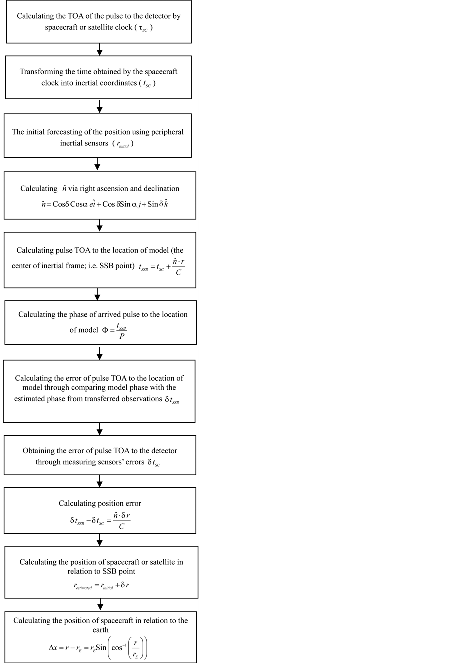

Figure 19. Three-dimensional positioning using three pulsars [22] .
An example of positioning using the algorithm above is as follows [22] :

If the pulse received is as shown above, and assuming that ,
,  , and
, and , then:

If the observed position is 4, and the TOA of the pulse to detector is 4, then:

The pulsar has turned twice in 4 seconds. Thus, frequency is 0.5, and period is 2. The pulse model will be:

The TOA of the pulse to the center of model is 8 seconds, and to the detector is 4. Therefore, the estimated phase for the model from the observation phases (2) will be:

Regarding the error of pulse TOA to the model, through comparing the obtained phase from the model with the estimated phase of the model from the observed pulse it can be concluded that:

Regarding sensor error, if the error of pulse TOA to detector is  the position error will be:

Considering the position error, the exact position will be:

Position Determination Algorithm 2

Velocity determination algorithm

Considering Einstein’s relativity theory, it is taken for granted that the spent time for the atomic clock in the spacecraft is different from the time spent in earth clock. Therefore, sometime transformations are to be conducted prior to using the above-mentioned algorithms, which will be dealt with in another article.
8. Conclusions
In this paper, three new algorithms for determining position and velocity of spacecraft or satellite in interplants and long space missions were presented. The first positioning algorithm is based on calculating the error of pulse TOA to detector, and then calculating the error of the obtained position. In the second positioning algorithm, the angle between pulsar and a planet with a certain position in satellite FOV is calculated. Satellite position in relation to earth is obtained using this information, and solving two equations with two unknown quantities. In the velocity determination algorithm, pulse TOA to detector, frequency of pulse arrival to model and detector, and light velocity are used. Attitude determination was not dealt with in this paper due to the abundance of methods in navigation in this regard (namely star tracker).
Many different references were referred to in writing this paper. The three algorithms suggested were not present in any of them however.
References
- Sheikh, S.I., Darryll, J.P., Ray, S.R., Wood, K.S., Lovellette, M.N. and Wol, M.T. (2006) Spacecraft Navigation Using X-Ray Pulsars. Journal of Guidance, Control and Dynamics, 29, 49-63. http://dx.doi.org/10.2514/1.13331
- Frommert, H. and Kronberg, C. (2005) The First Known Variable Stars. http://www.seds.org/~spider/spider/Vars/vars.html
- Hogg, H.S. (1984) Variable Stars. In: Gingerich, O., Ed., The General History of Astronomy: Volume 4, Astrophysics and Twentieth-Century Astronomy to 1950: Part A, Cambridge University Press, Cambridge, 73-89.
- Ghosh, P. (2007) Rotation and Accretion Powered Pulsars. World Scientific, Singapore City, 2.
- Longair, M.S. (1996) Our Evolving Universe. CUP Archive, 72.
- Longair, M.S. (1994) High Energy Astrophysics. Volume 2, Cambridge University Press, Cambridge, 99. http://dx.doi.org/10.1017/CBO9781139170505
- Reichley, P.E. and Downs, G.S. (1969) Observed Decrease in the Periods of Pulsar PSR 0833-45. Nature, 222, 229- 230. http://dx.doi.org/10.1038/222229a0
- Radhakrishnan, V. and Manchester, R.N. (1969) Detection of a Change of State in the Pulsar PSR 0833-45. Nature, 222, 228-229. http://dx.doi.org/10.1038/222228a0
- Reichley, P., Downs, G. and Morris, G. (1971) Use of Pulsar Signals as Clocks. NASA Jet Propulsion Laboratory Quarterly Technical Review, 1, 80-86.
- Reichley, P.E., Downs, G.S. and Morris, G.A. (1970) Time-of-Arrival Observations of Eleven Pulsars. The Astrophysical Journal, 159, L35-L40. http://dx.doi.org/10.1086/180473
- Reichley, P.E., Downs, G.S. and Morris, G.A. (1971) Second Decrease in the Period of the Vela Pulsar. Nature Physical Science, 234, 48-48.
- Rawley, L.A., Taylor, J.H., Davis, M.M. and Allan, D.W. (1987) Millisecond Pulsar 1937: A Highly Stable Clock. Science, 238, 761-765. http://dx.doi.org/10.1126/science.238.4828.761
- Ashby, N. and Allan, D.W. (1984) Coordinate Time On and near the Earth. Physical Review Letters, 53, 1858. http://dx.doi.org/10.1103/PhysRevLett.53.1858
- Downs, G.S. (1974) Interplanetary Navigation Using Pulsating Radio Sources. NASA TR N74-34150, October 1974, 1-12.
- Chester, T.J. and Butman, S.A. (1981) Navigation Using X-Ray Pulsars. NASA TR N81-27129, June 1981, 22-25.
- Wood, K.S. (1993) Navigation Studies Utilizing the NRL-801 Experiment and the ARGOS Satellite. In: Horais, B.J., Ed., Small Satellite Technology and Applications III, Society of Photo-Optical Instrumentation Engineers Proceedings, Bellingham, 105-116.
- Hanson, J.E. (1996) Principles of X-Ray Navigation. Ph.D. Dissertation, Department of Aeronautics and Astronautics, Stanford University, Stanford.
- Wood, K.S., Fritz, G., Hertz, P., Johnson, W.N., Kowalski, M.P., Lovellette, M.N., Wolff, M.T., Yentis, D.J., Bloom, E., Cominsky, L., Fairfield, K., Godfrey, G., Hanson, J., Lee, A., Michelson, P., Taylor, R. and Wen, H. (1994) The USA Experiment on the ARGOS Satellite: A Low Cost Instrument for Timing X-Ray Binaries. In: Siegmund, O.H. and Vallerga, J.V., Eds., EUV, X-Ray, and Gamma-Ray Instrumentation for Astronomy V, Society of Photo-Optical Instrumentation Engineers Proceedings, Bellingham, 19.
- Wood, K.S., Fritz, G., Hertz, P., Johnson, W.N., Lovellette, M.N., Wolff, M.T., Bloom, E., Godfrey, G., Hanson, J., Michelson, P., Taylor, R. and Wen, H. (1994) The USA Experiment on the ARGOS Satellite: A Low Cost Instrument for Timing X-Ray Binaries. In: Holt, S.S. and Day, C.S., Eds., The Evolution of X-Ray Binaries, American Institute of Physics Proceedings, Melville, 561-564.
- http://en.wikipedia.org/wiki/Pulsar.
- Sheikh, S.I. (1995) The Use of Variable Celestial X-Ray Sources For Spacecraft Navigation. Ph.D. Dissertation, Department of Aerospace Engineering, Maryland University, Maryland.
- Hanson, J., Sheikh, S., Graven, P. and Collins, J. (2008) Noise Analysis for X-Ray Navigation Systems. Proceedings of 2008 IEEE/ION Position, Monterey, 5-8 May 2008, 704-713.
NOTES

*Corresponding author.