International Journal of Astronomy and Astrophysics
Vol.3 No.3(2013), Article ID:36513,14 pages DOI:10.4236/ijaa.2013.33031
Are Uranus & Neptune Responsible for Solar Grand Minima and Solar Cycle Modulation?
Moonbeam Close, Narre Warren South, Melbourne, Australia
Email: gs_qad@hotmail.com
Copyright © 2013 Geoff J. Sharp. This is an open access article distributed under the Creative Commons Attribution License, which permits unrestricted use, distribution, and reproduction in any medium, provided the original work is properly cited.
Received April 7, 2013; revised May 9, 2013; accepted May 16, 2013
Keywords: Solar Grand Minimum; Solar Modulation; Angular Momentum; Uranus; Neptune; SSB; Barycentre
ABSTRACT
Detailed solar Angular Momentum (AM) graphs produced from the Jet Propulsion Laboratory (JPL) DE405 ephemeris display cyclic perturbations that show a very strong correlation with prior solar activity slowdowns. These same AM perturbations also occur simultaneously with known solar path changes about the Solar System Barycentre (SSB). The AM perturbations can be measured and quantified allowing analysis of past solar cycle modulations along with the 11,500 year solar proxy records (14C & 10Be). The detailed AM information also displays a recurring wave of modulation that aligns very closely with the observed sunspot record since 1650. The AM perturbation and modulation is a direct product of the outer gas giants (Uranus & Neptune). This information gives the opportunity to predict future grand minima along with normal solar cycle strength with some confidence. A proposed mechanical link between solar activity and planetary influence via a discrepancy found in solar/planet AM along with current AM perturbations indicate solar cycle 24 & 25 will be heavily reduced in sunspot activity resembling a similar pattern to solar cycles 5 & 6 during the Dalton Minimum (1790-1830).
1. Introduction
Solar system dynamics have been postulated as the main solar driver for many decades. Jose (1965) [1] was the first to associate a recurring solar system pattern of the 4 outer planets (179 years). Jose suggested this pattern correlates with the modulation of the solar cycle. New research via this study suggests that over the past 6000 years the 179 year cycle cannot be maintained and is closer to a 172 year cycle which aligns with the synodic period of Uranus & Neptune (171.44 years). Later Landscheidt (2003) [2] progressed the planetary influence theories further by associating quasi-cyclic negative torque readings or “zero crossings” (AM readings going below zero) that can occur near grand minima. It has been found since that the negative readings occur in the general region of most grand minima but such records are not a reliable method of predicting the timing and strength of grand minima at the solar cycle level.
Other studies detailed the orbit path of the Sun around the Solar System Barycentre (SSB) that showed a balanced trefoil pattern during times of “normal” solar cycles. Charvàtovà (2000) [3] shows this pattern or pathway as it moves to a disordered state during times of solar slowdown and are a direct result of the Uranus/Neptune conjunction of the era.
Theodor Landscheidt’s work has inspired both professional and citizen scientists. For example, Carl Smith (2007) [4] while researching Landscheidt’s work produced an AM graph using the JPL ephemeris (Figure 1). This graph for the first time clearly showed the detailed perturbations of solar AM that also coincide with past solar slowdowns along with the disordered solar path about the SSB. Carl Smith passed away in 2009 and to our knowledge was probably not aware of the hidden detail that was contained in his work, the Perturbed Angular Momentum curve holding the clue.
The perturbed curves on the solar AM graph (Figure 1) correspond with solar torque perturbations, which also alter the normal balanced solar path around the SSB. The solar velocity is also perturbed on a 172-year cycle (average) and a greater diversion between the orbital AM of the Sun and planets is observed. It is proposed through a spin orbit coupling mechanism resulting in varying solar equatorial rotation rate, the solar dynamo is reduced during these 172 year intervals.
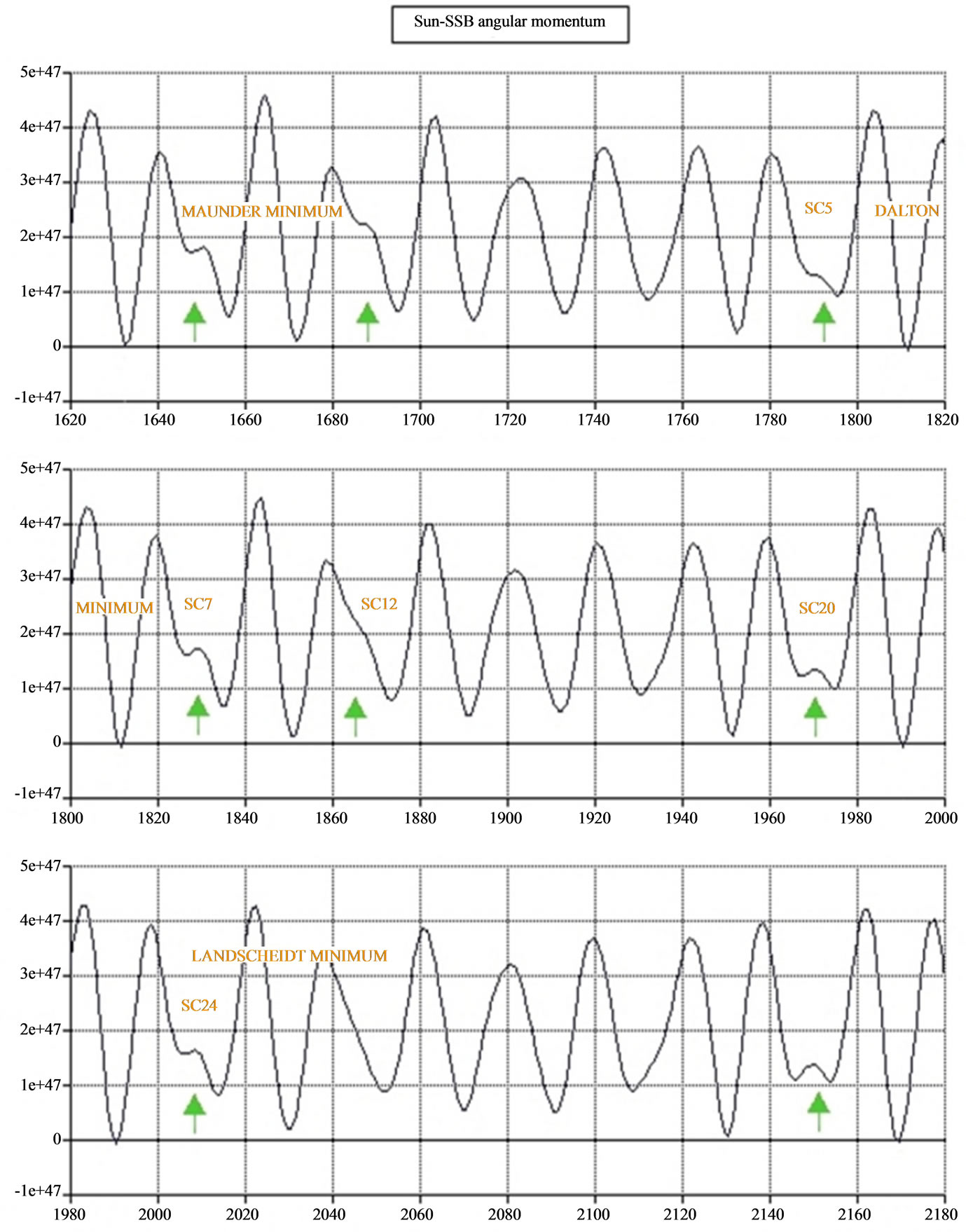
Figure 1. Detailed Solar Angular Momentum graph showing the perturbations (AMP events) at the green arrows. This graph is a modified example of Carl Smith’s original work that is based on JPL DE405 data. The green arrows and solar grand minima headings have been added. Carl Smith’s [4] original graph is displayed HERE Note: AM units of measure equate to gram-cm^2/sec.
2. Discussion—Grand Minima
The AM perturbations shown in Figure 1 are the result of the extra AM from the Uranus/Neptune conjunction. The timing in relation to the Jupiter/Saturn opposition provides the different perturbation shapes that can be measured via the relevant planet angles and categorised into two groups. Perturbations occurring on the down slope are denoted “Type A” and those on the up slope “Type B” (down slope = right hand side of peak).
Type B occurrences coincide with weaker solar slowdowns and are more common before 1000AD and the Medieval Warm Period (MWP). Almost all perturbations throughout the past 6000 years coincide with solar downturns that vary in intensity.
During the past 750 years strong Type A perturbations are evident on the AM graph (Figure 1). Coinciding with the strong Type A multiple appearances is one of the greatest sustained periods of grand minima of the Holocene (Little Ice Age 1300 - 1870 approx.). The Type A perturbations all have the same planetary configuration, but with slightly differing planet angles (Figure 2).
Type A perturbations have a positive Saturn angle, the higher the Saturn angle the higher the perturbation height on the AM graph. Type B perturbations always display a negative Saturn angle (Figure 2). During each conjunction of Uranus & Neptune, Jupiter & Saturn have multiple oppositions. Depending on the planet positions of the era this can result in normally 3 - 4 Angular Momentum Perturbations (AMP) events for each Uranus/Neptune conjunction. The midpoint of these AMP groups displays a 172-year average spacing. The Sporer Minimum (1400 - 1600 approx.) has 2 strong AMP events, and 2 medium AMP events that coincide with one of the longest and
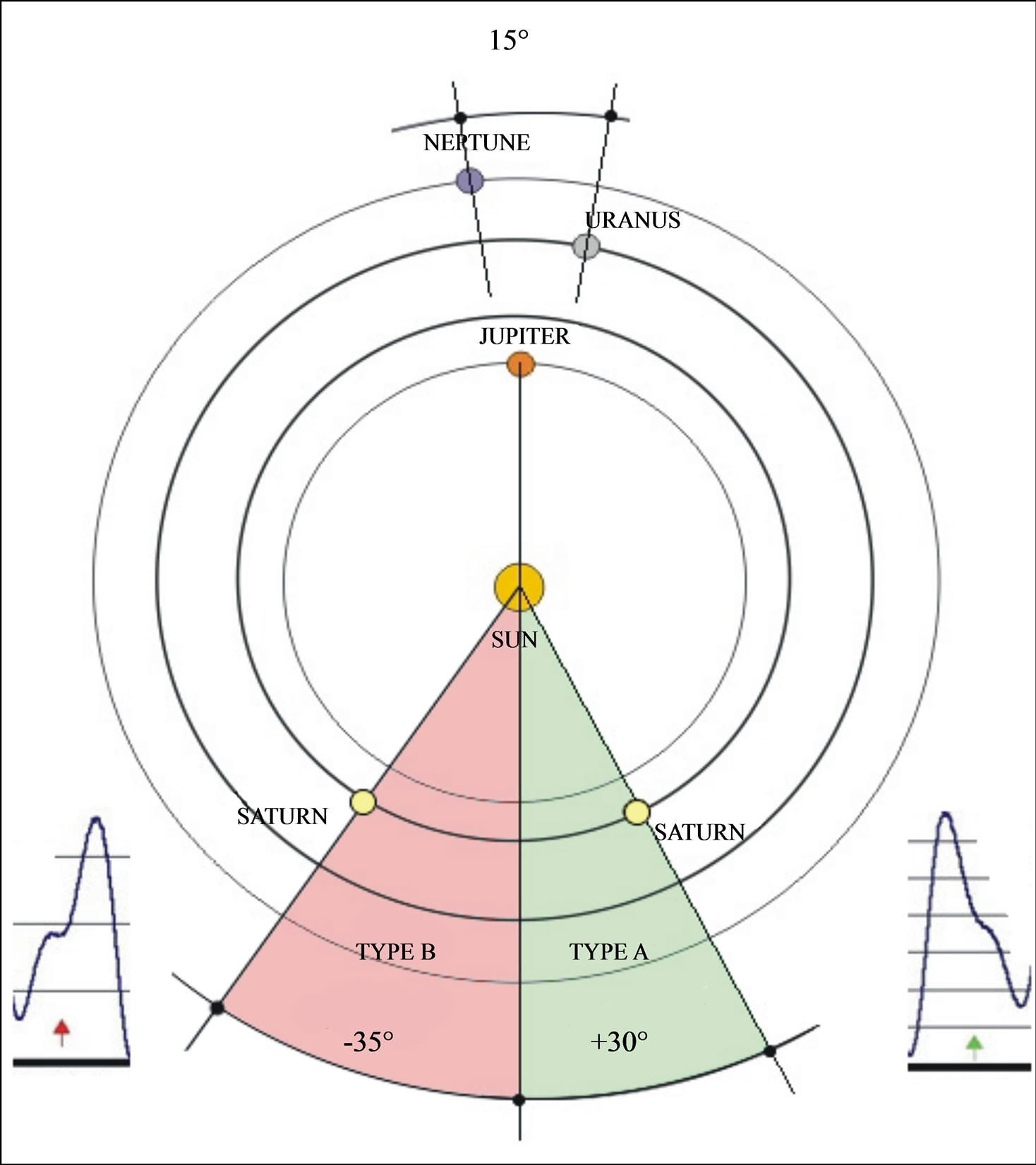
Figure 2. Typical planet positions demonstrating strong Types A & B perturbations. The Type A example is taken from near the centre of the Sporer Minimum (1472). Type B events coinciding with less reduction of solar activity compared with Type A events of similar angle (reverse).
deepest grand minima of the Holocene.
Type A AMP events have a major impact on the inner loop trajectory of the Sun in its orbit around the SSB. The Sun normally follows two distinct loops around the SSB (Figure 3) with each loop lasting approximately ten years. A shallow inner loop is evident when Jupiter & Saturn are in opposition and a much wider loop when Jupiter & Saturn are in conjunction. During strong Type A AMP events the inner loop path is greatly extended pushing the Sun out of its normal balanced trefoil pattern whereas the normal trefoil pattern returns the Sun to near the SSB on the inner loop path. The AMP event shows the path greatly extended from the SSB, the inner loop is trying to be an outer loop. Type B AMP events affect the outer loop of the Sun’s path, which has the effect of reducing the distance travelled away from the SSB. Accompanying the AMP events is usually a zero crossing (solar AM goes below zero) where Saturn, Uranus &
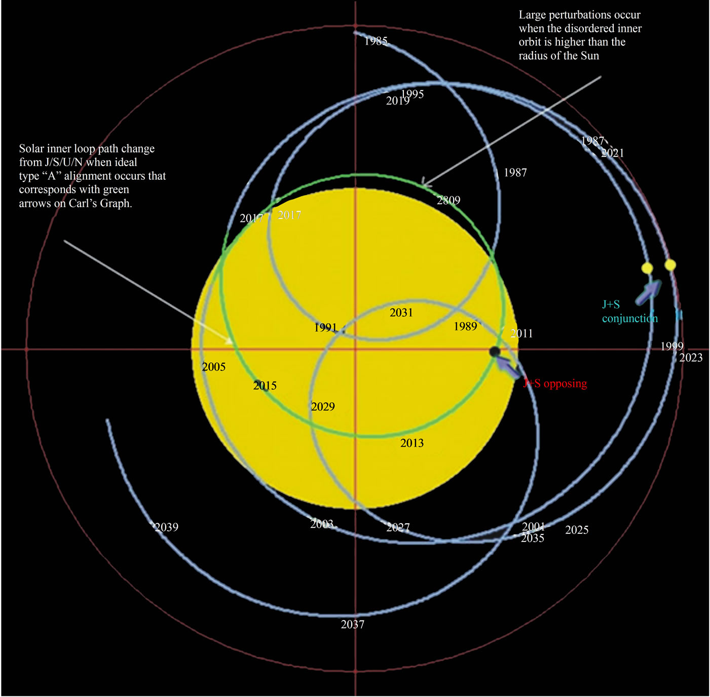
Figure 3. The path of the Sun shows the two distinct loops around the SSB (centre point). The extended inner loop beginning around 2005 coinciding with a reasonably strong Type A event. Solar cycle 24 is predicted to be the first grand minimum cycle. The sunspot records since 1650 suggest that 2 solar cycles can be affected by strong Type A events, there is speculation that the Hale cycle is interrupted and follows a 22-year-period. An animated movie of the path taken can be viewed at http://www.landscheidt.info/images/sim.swf.
Neptune are in conjunction with Jupiter opposing. This places the Sun right on the SSB, or indeed on the other side of the SSB. The zero crossings can occur either side of an AMP event.
The Carbon 14 (14C) record for the Holocene is a reliable solar proxy record. Recent Beryllium 10 (10Be) isotope records derived from ice cores by Steinhilber, Beer, Frolich (2009) [5] confirm the accuracy of the 14C record (Figure 4). During the 11,500 years of the Holocene a regular pattern of solar downturns can be observed which vary in intensity. The 14C records used in this report are originally from the INTCAL98 (Stuiver, et al., 1998b) [6] study and further extended by Solanki et al. (2004) [7] and Usoskin, Solanki & Kovaltsov (2007) [8]. The 14C values are compared with the AMP group centre values (Figure 5). The isotope data show a strong correlation with each individual AMP group in timing and strength. Each AMP group centre has the relevant planet angles recorded including the orientation of Uranus/ Neptune (Figure 6). The Figure 6 refers to Figure 5" target="_self"> Figure 5 AM group centres. Most AMP groups are comprised of three to four separate AMP events separated by approx. 40 years.
The planetary angles taken at the AMP events (Figure
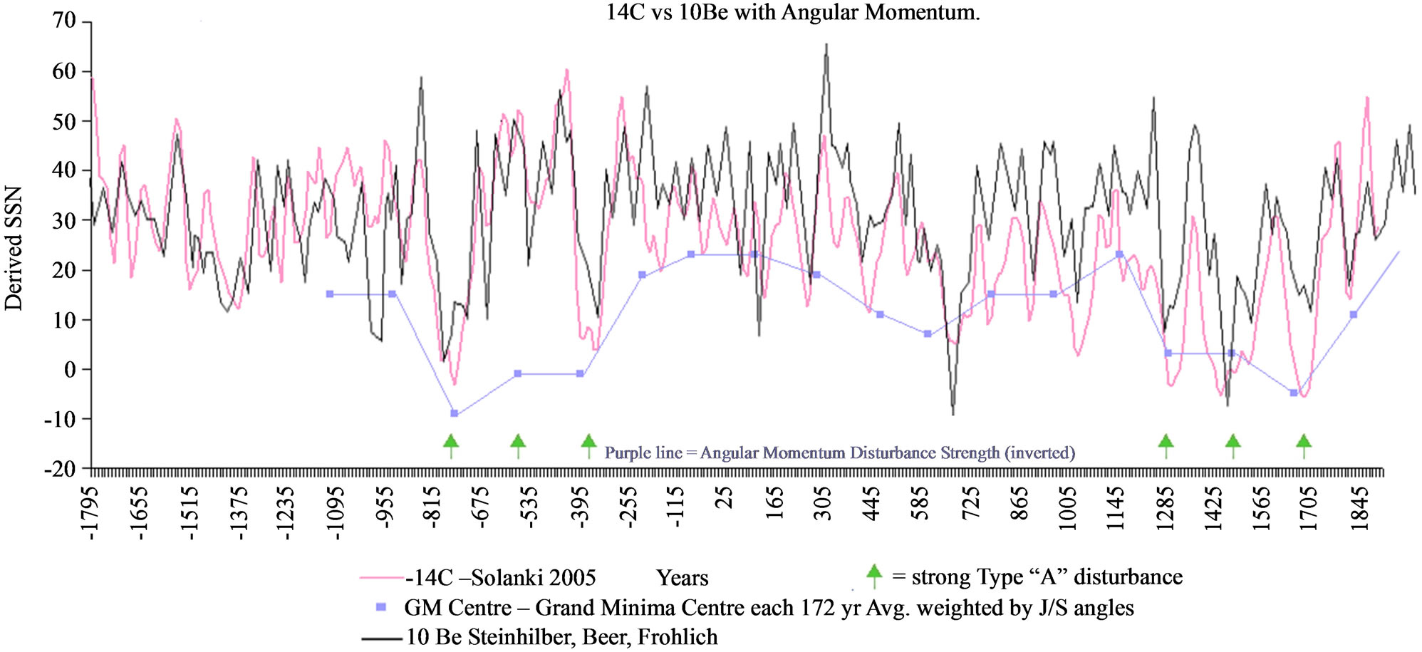
Figure 4. Comparison of 14C and 10Be isotope records. The purple line is a representation of the AMP group strength (individual AMP events are summed to form group totals, details follow in later section) with each point representing the AMP centre. A full size image can be viewed at http://www.landscheidt.info/images/solanki_sharp.png. The isotope plots are a graphical comparison of Solanki et al. (2004) [7] & Steinhilber et al. (2009) [5].
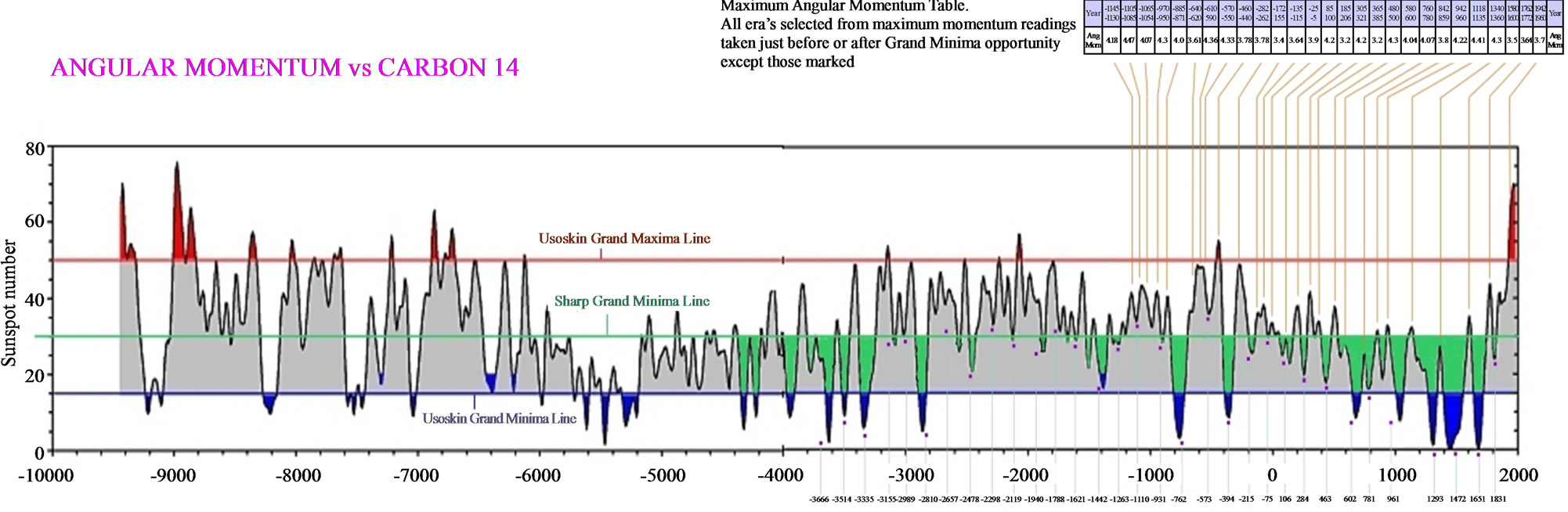
Figure 5. Graphical representation modified from the Usoskin et al. (2007) [8] solar proxy report. Usoskin determined that grand minima occur under 15SSN (derived SSN figures, blue line) that isolates Dalton Minimum type events. By raising the bar (green line) the repeating pattern of grand minima is observed. The middle AMP event per group is shown below the date axis with the peaks in AM shown at the top of the graph. Strong AMP groups coinciding with deep Grand Minima shown below blue line. A full size image can be viewed at http://www.landscheidt.info/images/c14nujs1.jpg.
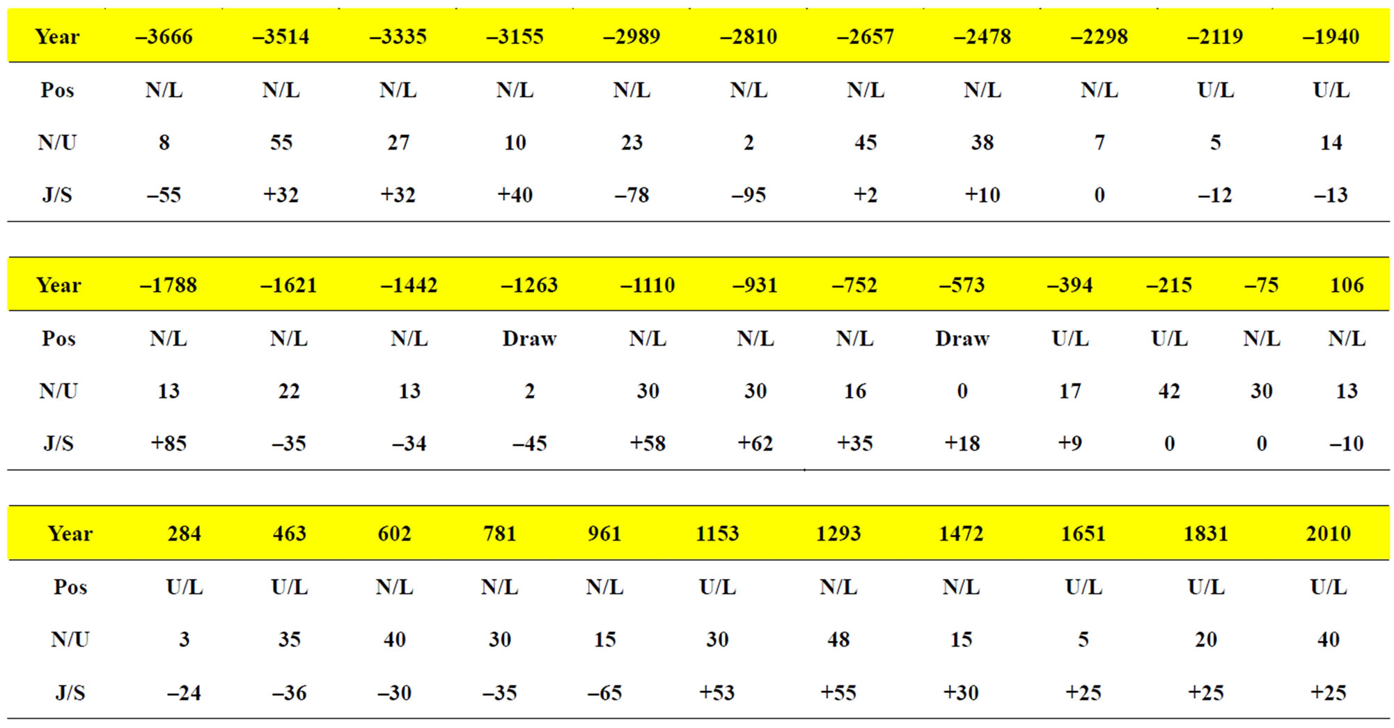
Figure 6. Planet angle tables referring to Figure 5 displaying the middle AMP event per 172 year average period. Pos = relative Uranus/Neptune position i.e. Neptune leading Uranus etc. N/U = angle measured between Neptune & Uranus. J/S = angle measured away from Jupiter/Saturn opposition.
6) providing a statistical measurement that can be compared with the AMP events and Figure 1. The depth of the solar downturns shown on the 14C graphs coinciding with the planet angles and observed AMP events, deep troughs aligning with strong Type A events and sustained periods of strong solar activity aligning with periods of weaker Type B events. Type A events can also be weak depending on the planet angles. Type B events occurring before 1000AD are a result of the changing planet angles that move slowly over long periods of time. The overall background shape of the 14C graph coincides with the occurrence and strength of Types A & B events. During times of multiple sustained Type B events, each 172 year cycle group can carry more than 3 events as observed in Figure 7.
Figure 7 shows each individual AMP event making up each AMP group, the strength of each disturbance coinciding with the relevant planet angles. Type A events with a J/S angle around +30 degree and N/U angle of 15 degree providing the strongest downturns, Type B&A events with a J/S angle near zero degree or 180 degree providing the weakest downturn. Weak AMP events coincide with the Medieval Warm Period 950AD-1250AD (Figure 8).
The Sporer Minimum (Figure 9) displayed the longest period of solar inactivity across the Little Ice Age coinciding with 3 strong Type A events and 1 Type B event. The last two AMP events during the Maunder Minimum being stronger than the initial AMP event occurring around 1610. Also see Figures 1 and 8.
3. Determining AMP Strength
The purple line shown on Figure 4 is a representation of the AMP strength of the era that follows the general trend of solar activity. The method used (Figure 10) is a preliminary method using visual observation of each disturbance of the graph period. Figure 1 displays the different types of AMP events that cycle in groups every 172 years (average). These disturbances always line up with periods of solar downturn.
The Solanki/Steinhilber [5,7] data shows regular solar downturns that vary in intensity, by observing the shapes of the AMP events that align with these downturns we are able to see a pattern that is repeatable.
There are rare occasions of strong Type A AMP events that do not cause solar activity reduction or perhaps not as low as expected, when not meeting the Wilson Test described in Wilson et al. (2008) [9] (Figure 11). This test states that for an AMP event to fully utilize the disturbance, the Jupiter/Saturn opposition or conjunction must happen before cycle maximum (to achieve a cycle with less than 80SSN). This has been tested over the sunspot record but is not available for accurate testing beyond this point as the cycle maximum date is not known. 1830 and –530 are probable examples of this phenomena, during 1830 the Jupiter/Saturn conjunction occurred before cycle maximum. AMP events need to occur well before cycle maximum to achieve full impact.
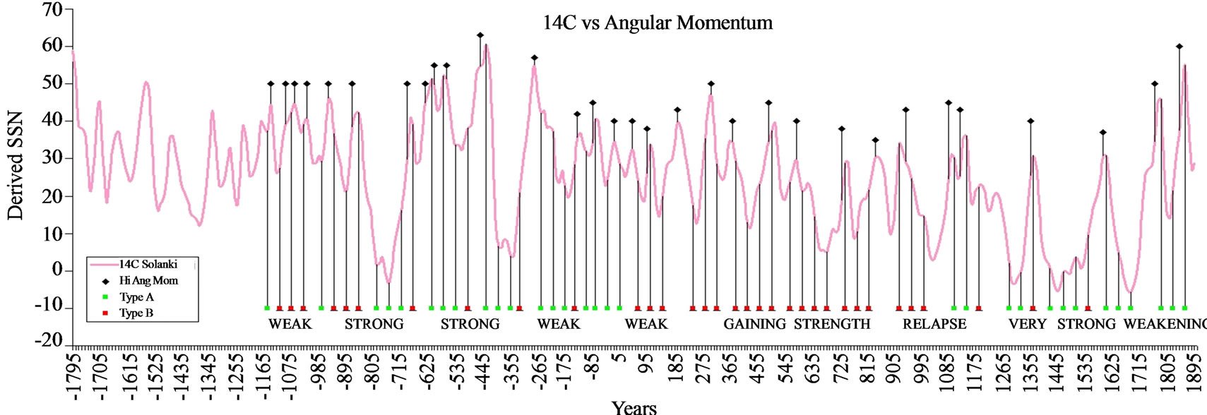
Figure 7. Individual AMP events plotted directly onto the Solanki data [7]. As each conjunction of Uranus & Neptune has a varying Jupiter/Saturn position, the strength of each individual AMP event along with the AMP group total changes over the millennia. This can be represented as the AM power curve of the Holocene. A full size image can be viewed at http:// www.landscheidt.info/images/solanki_sharp_detail.jpg. The spreadsheet with original Solanki data [7] with AMP events is available at http://www.landscheidt.info/images/solanki_sharp.xls.
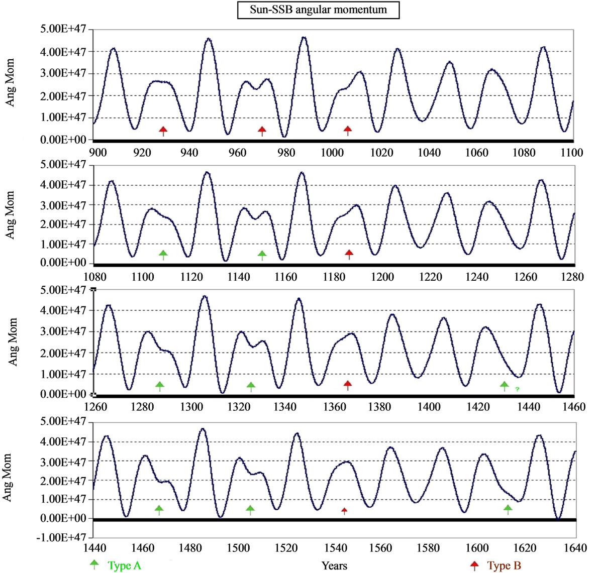
Figure 8. Solar AM graph depicting the period from 900AD - 1640AD. The change in Type A dominance shown after 1100AD. The MWP possibly being the only period during the Holocene not to be affected by the recurring 172 years AMP pattern. This is a time of transition moving from very weak Type B occurrence to a strengthening Type A dominance. The AMP events at 930 & 970 are midway between Types A & B. Note: AM units of measure equate to gram-cm^2/sec.
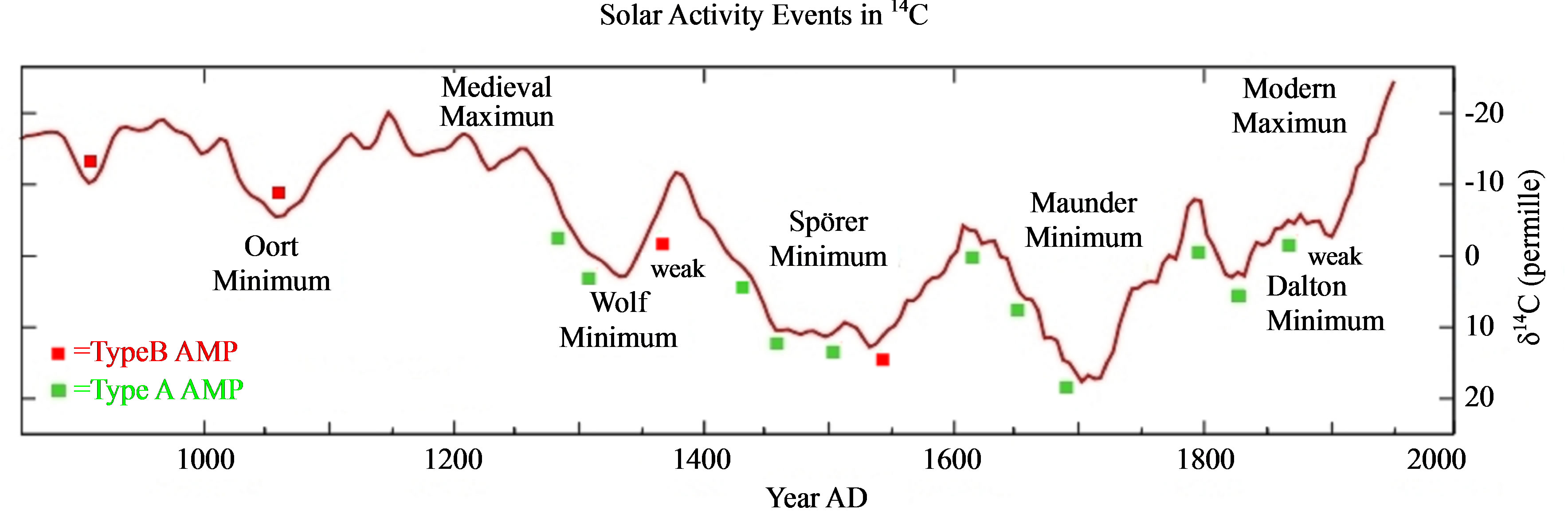
Figure 9. Carbon 14 graph (Wikipedia) with the AMP events overlaid.
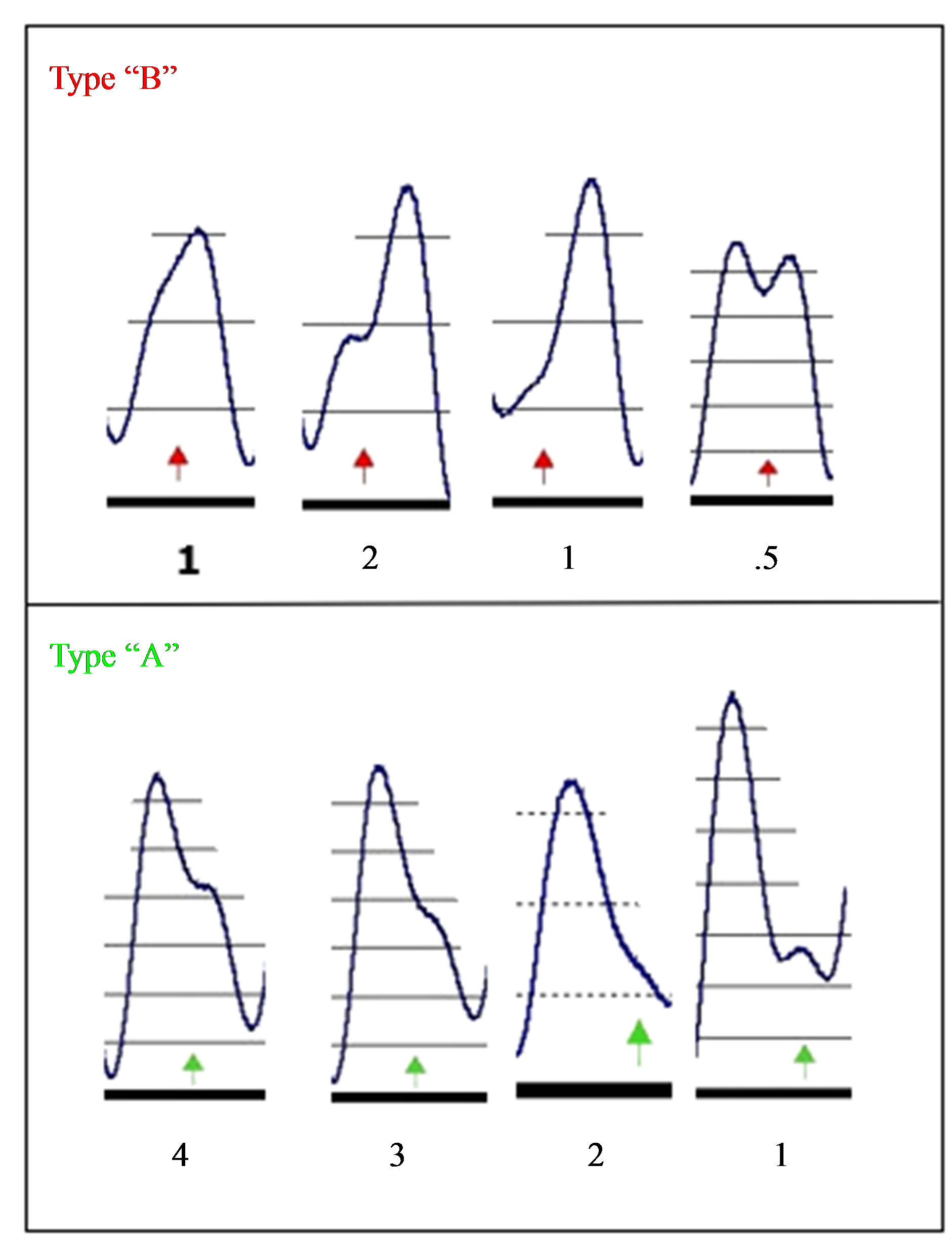
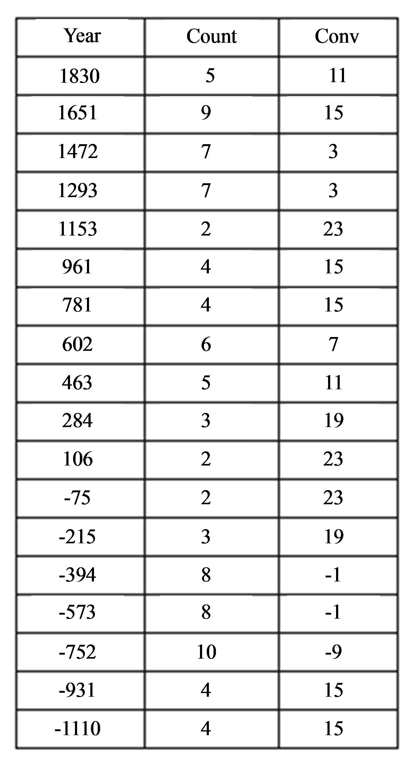
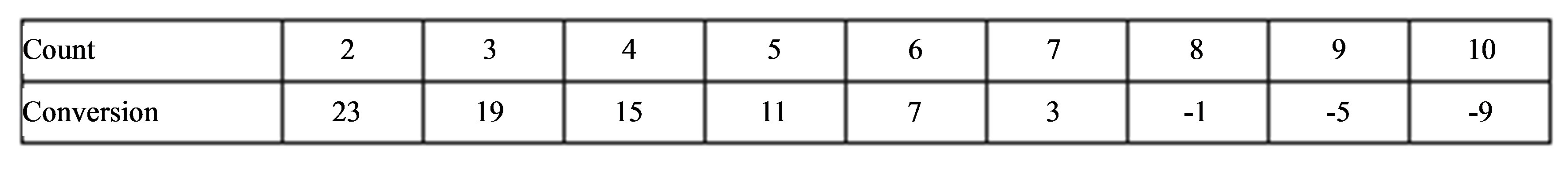
Figure 10. Charts showing the AMP strength quantification method. Each count unit corresponding with 4 units of Usoskin [8] derived SSN units. Future quantification methods involving accurate planet angles would provide more detail.
By matching the AMP event shapes on the AM graphs with solar downturn strength each disturbance can be quantified. AMP events that align with deep grand minima (on a constant basis throughout history) get the highest score and also show the same shape or perturbation.
4. Discussion—Solar Cycle Modulation
Solar cycle strength depicted by SSN (smoothed sunspot number) follows a recurring wave of power that follows the overall AM values. The AM wave displays a peak at the Uranus/Neptune conjunction and the corresponding trough at the Uranus/Neptune opposition, Scafetta (2009, 2010) [10] also recognized this trend in his work dealing with the celestial origin of climate oscillations. The SSN record of the past 400 years when matched with this wave shows a strong correlation. The AMP events that
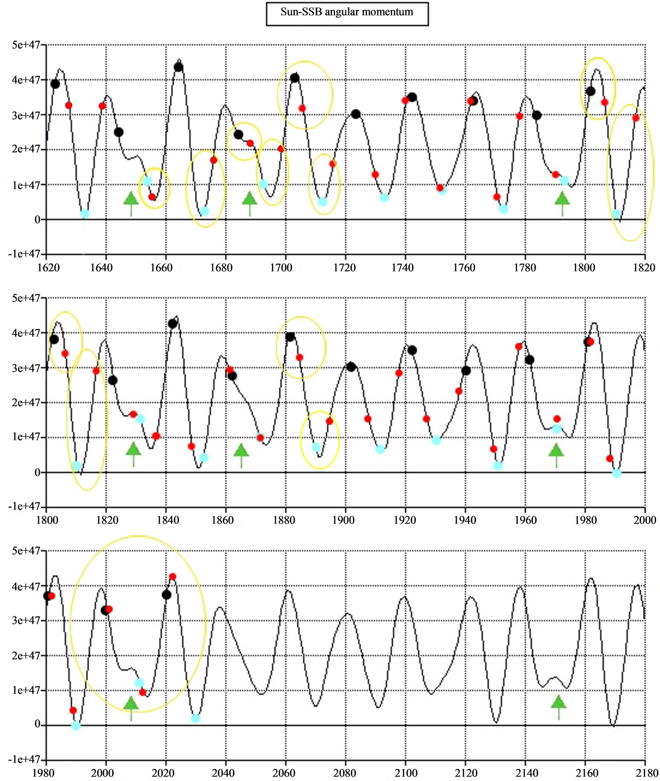
Figure 11. Wilson’s Test. Black dots are Jupiter/Saturn together, Blue dots Jupiter/Saturn opposed, and Red dots are solar cycle maxima, reduced solar activity occurs when a black or blue dot occurs in between cycle minimum and before cycle maximum. 1830 & 1790 does not pass the test. The yellow circles comply with Wilson’s Test. Note: AM units of measure equate to gram-cm^2/sec.
always occur at different intensities and length near the AM maximum interrupt the correlation and work as a separate process. The AM sine wave is also seen as a background solar engine that affects cycle modulation (SSN) but not the length of the cycle. Other processes determine the length of each solar cycle.
The Damon Minimum (1856-1913) is sometimes described as a grand minimum and is most likely an example of a low sunspot cycle/s affected by low AM at the time of the Uranus/Neptune opposition and not a true grand minimum. AMP events are not observed during these intervals with only low AM recorded. The AMP event is thought to create a “phase catastrophe” situation that perhaps is responsible for reported monopolar solar pole readings of the Maunder Minimum by Callebaut et al., (2007) [11]. The monopolar position is effectively providing the majority of sunspot activity to a single solar hemisphere. The monopolar position being described as a prolonged period where the solar poles have the same polarity as a result of only one pole reversing polarity during the Hale cycle. These events need to be accommodated when comparing the AM modulation versus the sunspot cycle modulation. The monopolar disturbance to the normal Hale cycle could explain the occurrence of twin low cycles paired during grand minima even though the second cycle is not perturbed. The poles require the extra cycle to maintain the normal synchronised state. The key point being that low cycles can be a result of low AM without experiencing “phase catastrophe” conditions. Grand minima occur during the higher part of the AM wave.
The AM graphs show a sine wave of AM modulation (around 10 years), the low points are considered as important as the high points. While a direct mechanical link between AM modulation and solar cycle modulation remains theoretical there is a direct example of some physical connection. The solar velocity (Figure 12) around the SSB is absolutely linked to the AM sine wave that provides a roughly decadal acceleration/deceleration phase.
To visualise the importance of the low points in relation to the high points of the AM graph, a centre point needs to be determined and the values recorded under that centre point are inverted. This provides a true reading of the AM strength (Figures 13 and 14). For the past 400 years an AM reading of 2E + 47 (gram-cm^2/sec) was used from Carl Smith’s data as the centre point.
5. Angular Momentum Data Formula
The original Carl Smith AM data [4] is referenced and validated by independent analysis carried out by G. E. Pease using JPL DE405 coordinates and the following standard AM formula:
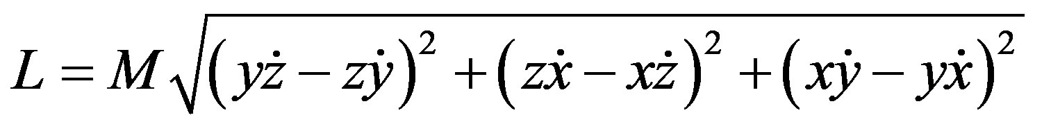
M is the Mass of the Sun in kilograms. x, y, z, xdot, ydot, zdot must be converted from kilometres and km/sec to metres and metres/sec to get m^2ks units. The equation yields the absolute value of L, using the instantaneous cross products of the body’s position and velocity vectors (Figure 15).
6. Proposed Mechanical Link via Spin Orbit Coupling
A spin orbit coupling mechanism has been discussed by Wilson et al. (2008) [9] which translates into a varying solar equatorial rotation speed, enabling changes to the solar dynamo and the meridional flows. Solar equatorial rotation rate changes have been recorded by Javaraiah (2003) [12] based on sunspot movement records.
Total Angular Momentum is the combination of orbital
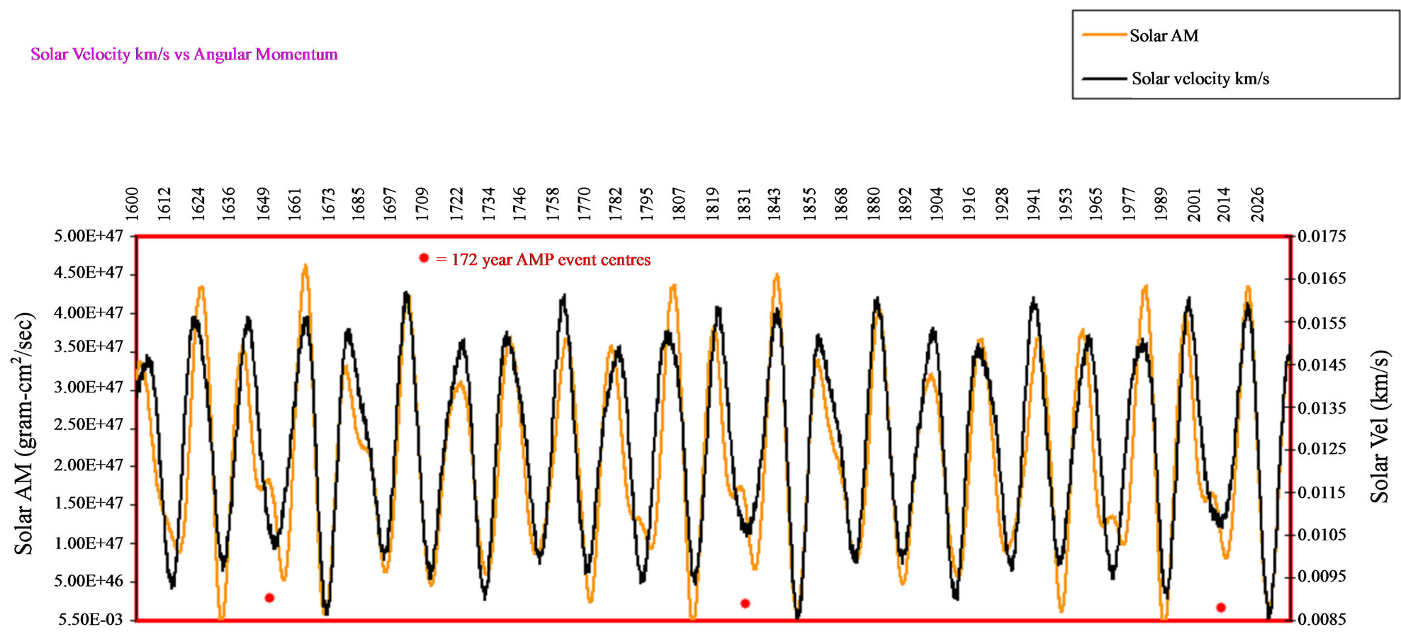
Figure 12. Solar AM values matched with solar velocity. The red dots displaying the 172-year centre of the AMP groups. Note the repeating pattern of change in velocity. Data source: Jet Propulsion Laboratory.
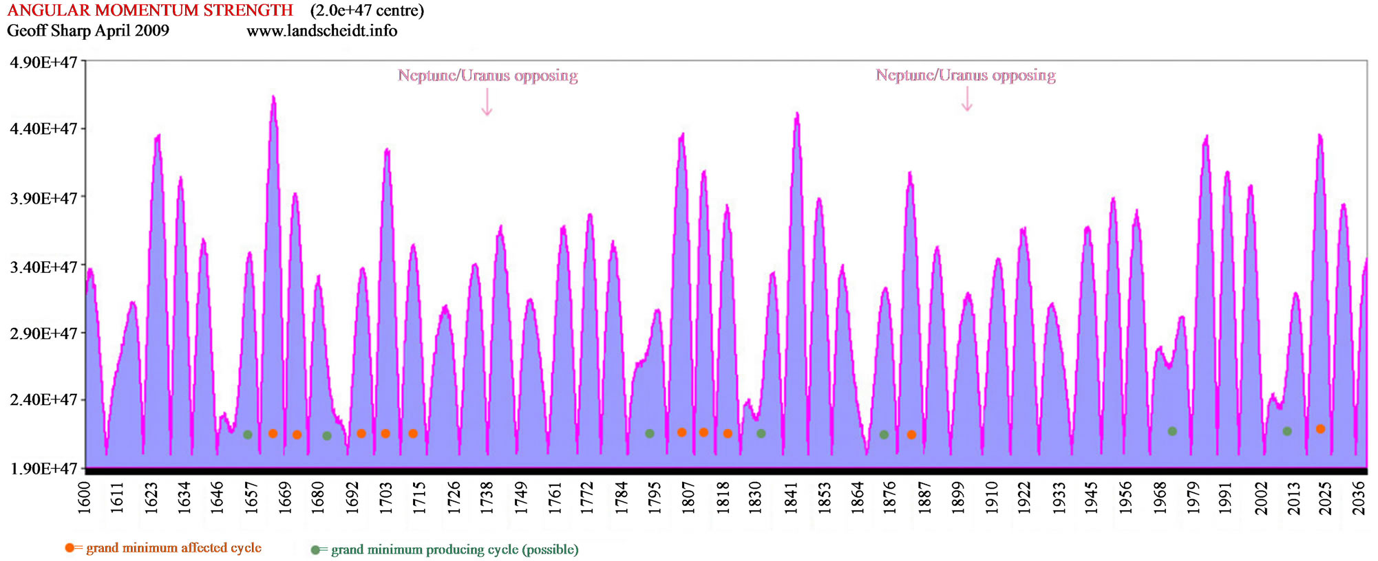
Figure 13. Manipulated Solar AM graph using Carl Smith’s original data [4] with all points on Figure 1 below 2E + 47 inverted. High and low AM extremes on Figure 1 are considered of equal importance, with high and low AM corresponding with strong solar cycles (outside of AMP events). High AM is linked with larger outer loop paths and lower AM linked with tighter inner loop paths towards the SSB as seen in Figure 3.
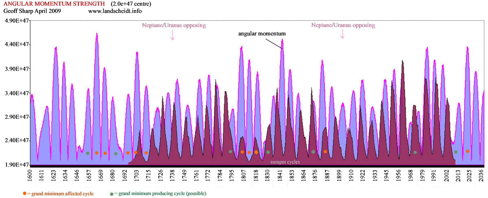
Figure 14. The values of Figure 13 are compared with the SIDC Smoothed Sunspot Number (SSN) values (overlaid graphically). Once allowing for AMP events and the coinciding low solar amplitude, the derived AM strength follows the SIDC sunspot record.
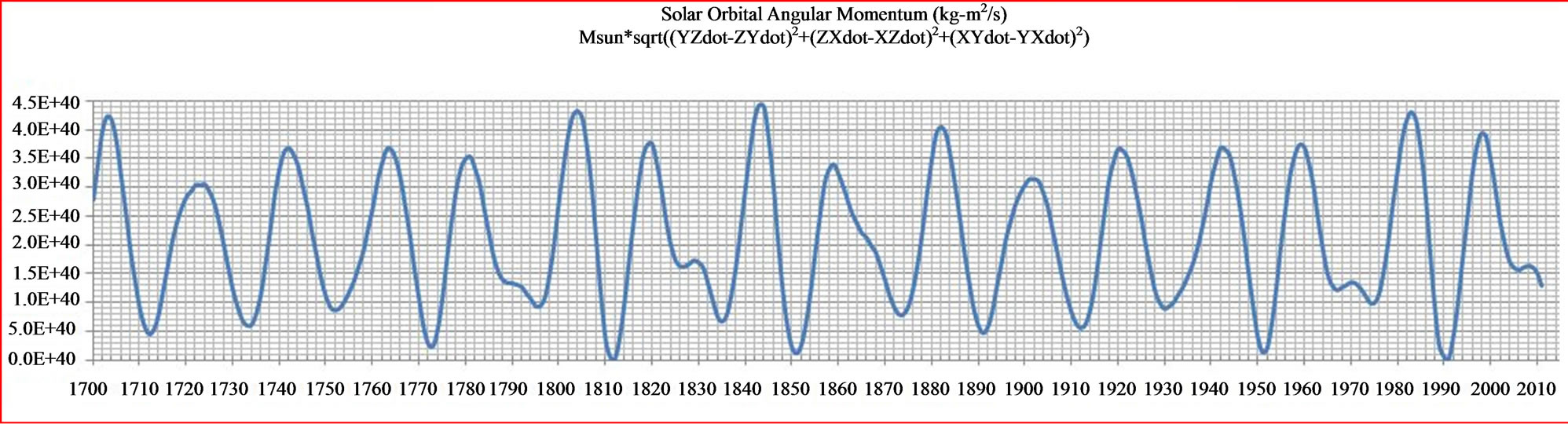
Figure 15. G. E. Pease AM graph depicting the same AMP events and timing as the Smith AM graph. The G. E. Pease graph using JPL DE405 xyz coordinate data and the above formula to produce the same AM outcomes as Figure 1.
AM and spin AM. The laws of AM conservation allow a “trade off” between orbital AM and spin AM. Each body in the solar system has its own orbital AM that can be calculated using the standard formula:

If there is a discrepancy between solar orbital AM and planet/body orbital AM the laws of AM conservation would allow changes to a body’s spin AM. This could result in a varying solar equatorial rotation rate.
To perform this task all the solar system planets and the asteroids Ceres, Juno, Vesta, Pallas, Eugenia, Siwa & Chiron have been included to arrive at a total planet AM. Data coordinates were taken from the JPL DE405 ephemeris.
To compare planet AM with solar AM the inertial frame should be the same. The JPL DE405 heliocentric planetary coordinates are referred to the solar system barycentric inertial frame rather than the heliocentric inertial frame, which required a transformation of our computed planetary angular momenta to the heliocentric inertial frame. The planet AM was calculated using heliocentric coordinates, the solar data was calculated using the SSB as the axis point (barycentric), then the solar AM is subtracted from the planet AM to achieve the same inertial frame.
The following graph (Figure 16) displays a divergence between solar and planet orbital AM. A future study will be performed with G.E. Pease further outlining this procedure. Extending this graph back over the whole Little Ice Age may prove interesting, possibly showing us another method of identifying solar slow down by studying the planetary AM and its relationship with solar AM.
Some big questions remain.
7. Conclusions and Predictions
The correlation of the inverted AM values with the existing sunspot record, along with the quantification of AMP events provides a platform for future sunspot prediction out to 3000AD. Cycles 24 & 25 are predicted to be less than 50SSN using the Layman’s Sunspot Count (based on the SIDC values but ignoring specks rated lower than 23 pixels). Solar cycle 20 was the first stage of the current AMP group that failed to generate a full grand minimum. This stems from the very weak AMP event caused by the late timing of the Uranus/Neptune conjunction and the failed Wilson’s Test. The current AMP group does not display a third event that is extremely rare and hence will allow a modest recovery during solar cycle 26 (Figure 17). Looking out further, the next 1000 years do not show any major chances for deep grand minima that should provide stable conditions for future generations, not withstanding the possible entry into the next ice age (Figure 18).
Solar cycle 24 will need to reach maximum after March 2011 to comply with the Wilsons Test.
Further information on the Layman’s Sunspot Count can be found at: http://www.landscheidt.info/?q=node/50.
8. Acknowledgements
Special thanks go to G. E. Pease for confirming Carl Smith’s AM data and for the advice and input on inertial frames.
The author would also like to thank Nicola Scafetta for providing advice and the initial peer review.

Figure 16. Differences in orbital AM become clear when viewed in the correct inertial frame. Note the near constancy (smaller range of deviation from top to bottom) of the Planet AM after subtracting the solar AM. The Planet AM is now constant to six significant figures, whereas it was only constant to three significant figures before the inertial frame transformation. We believe the residual variations in the seventh and higher significant digits may be the result of spin orbit coupling between the planetary orbits and solar rotation.
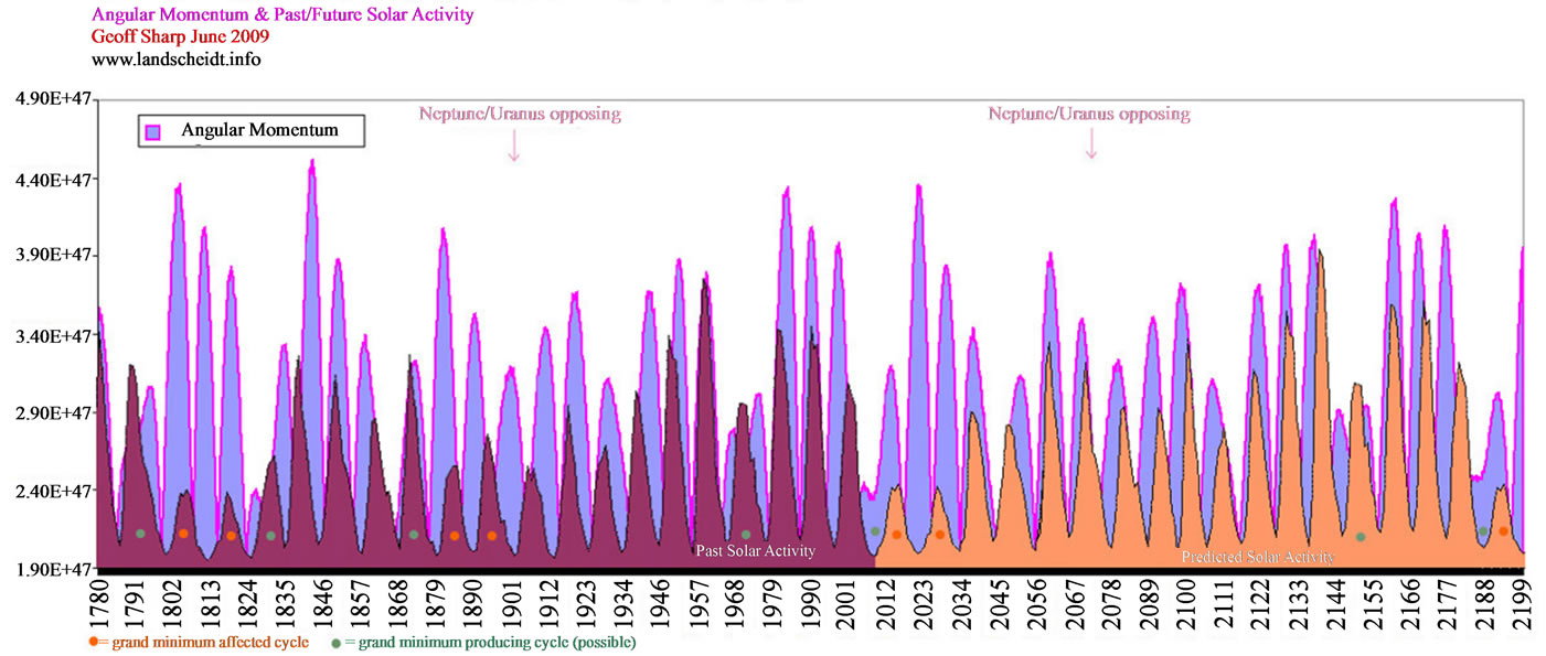
Figure 17. 200-year solar cycle prediction. The trough in the sunspot record coinciding with the opposition of Uranus & Neptune in past records and is expected to remain the same. Solar proxy records do not show high solar activity during times of low AM (Figures 5 & 7). The length of each future solar cycle remains unknown and predicted solar cycles should be taken as a guide with the overall trend being important. AM timing does not seem to be related to solar cycle timing. Predictions are based on overall AM strength.
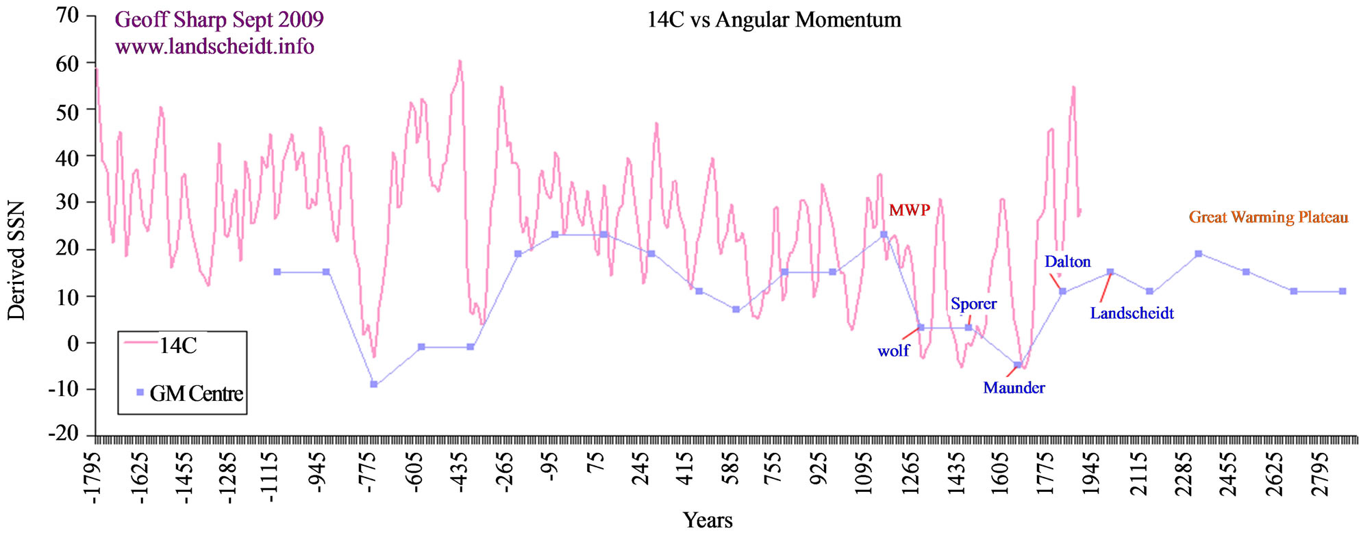
Figure 18. Earth’s future climate based on the projected solar activity using the same method as described in the chapter headed “Determining AMP Strength”. Deep grand minima are not expected. GM centre refers to the central AMP event occurring each 172 years on average, all AMP events in that group are totalled.
The SIM diagram (Figure 3) produced with software made available by Carsten Arnholm.
The data and main concepts were first published online 6 November 2008 at http://landscheidt.wordpress.com/2008/ 11/06/are-neptune-and-uranus-the-major-players-in-solar-grand-minima/. This document is a summary of many articles published at http://landscheidt.wordpress.com and http:// www.landscheidt.info.
REFERENCES
- P. Jose, “Sun’s Motion and Sunspots,” Astronomical Journal, Vol. 70, 1965, pp. 193-200. doi:10.1086/109714
- T. Landscheidt, “New Little Ice Age Instead of Global Warming,” Energy and Environment, Vol. 14, No. 2-3, 2003, pp. 327-350.
- I. Charvàtovà, “Can Origin of the 2400-Year Cycle of Solar Activity Be Caused by Solar Inertial Motion?” Geophysical Institute AS CR, Bocnõ II, Czech Republic, 2000.
- C. Smith, “Angular Momentum Graph,” 2007. http://landscheidt.wordpress.com/2007/06/01/dr-landscheidts-solar-cycle-24-prediction http://landscheidt.wordpress.com/6000-year-ephemeris
- F. Steinhilber, J. Beer and C. Frohlich, “Total Solar Irradiance during the Holocene,” Geophysical Research Letters, Vol. 36, No. 19, 2009, p. L19704. doi:10.1029/2009GL040142
- M. Stuiver, P. J. Reimer, E. Bard, J. W. Beck, G. S. Burr, K. A. Hughen, B. Kromer, G. McCormac, J. van der Plicht and M. Spurk, “INTCAL98 Radiocarbon Age Calibration, 24,000#0 cal BP,” Radiocarbon, Vol. 40, 1998, p. 1041#83.
- S. K. Solanki, I. G. Usoskin, B. Kromer, M. Schussler and J. Beer, “Unusual Activity of the Sun during Recent Decades Compared to the Previous 11,000 Years,” Nature, Vol. 431, No. 7012, 2004, pp. 1084-1087. ftp://ftp.ncdc.noaa.gov/pub/data/paleo/climate_forcing/solar_variability/solanki2004-ssn.txt
- I. Usoskin, S. Solanki and G. Kovaltsov, “Grand Minima and Maxima of Solar Activity: New Observational Constraints,” Astronomy & Astrophysics Manuscript No. 7704, 2007.
- I. Wilson, B. Carter and I. A. Waite, “Does a Spin-Orbit Coupling between the Sun and the Jovian Planets Govern the Solar Cycle?” Publications of the Astronomical Society of Australia, Vol. 25, No. 2, 2008, pp. 85-93. http://www.publish.csiro.au/?act=view_file&file_id=AS06018.pdf doi:10.1071/AS06018
- N. Scafetta, “Empirical Evidence for a Celestial Origin of the Climate Oscillations and Its Implications,” Journal of Atmospheric and Solar-Terrestrial Physics, Vol. 72, No. 13, 2010, pp. 951-970. http://yosemite.epa.gov/ee/epa/eed.nsf/vwpsw/360796B06E48EA0485257601005982A1#video doi:10.1016/j.jastp.2010.04.015
- D. Callebaut, V. Makarov and A. Tlatov, “Monopolar Structure of the Sun in between Polar Reversals and in Maunder Minimum,” Advances in Space Research, Vol. 40, No. 12, 2007, pp. 1917-1920.
- J. Javaraiah, SoPh, Vol. 212, 2003, p. 23.