Advances in Chemical Engineering and Science
Vol. 2 No. 2 (2012) , Article ID: 18900 , 11 pages DOI:10.4236/aces.2012.22029
Studies on the Evaporation Regulation Mechanisms of Crude Oil and Petroleum Products
Spill Science, Edmonton, Canada
Email: fingasmerv@shaw.ca
Received January 12, 2012; revised February 18, 2012; accepted March 20, 2012
Keywords: Oil Evaporation; Petroleum Evaporation; Boundary-Layer Regulation
ABSTRACT
Various concepts for oil evaporation prediction are summarized. Models can be divided into those models that use the basis of air-boundary-regulation or those that do not. Experiments were conducted to determine if oil and petroleum evaporation is regulated by the saturation of the air boundary layer. Experiments included the examination of the evaporation rate with and without wind, in which case it was found that evaporation rates were similar for all wind conditions and no-wind conditions. Experiments where the area and mass varied showed that boundary-layer regulation was not governing for petroleum products. Under all experimental and environmental conditions, oils or petroleum products were not found to be boundary-layer regulated. Experiments on the rate of evaporation of pure compounds showed that compounds larger than Decane were not boundary-layer regulated. Many oils and petroleum products contain few compounds smaller than decane, and this explains why their evaporation is not air boundary-layer limited. Comparison of the air saturation levels of various oils and petroleum products shows that the saturation concentration of water, which is strongly air boundary-regulated, is significantly less than that of several petroleum hydrocarbons. Lack of air boundary-layer regulation for oils is shown to be a result of both this higher saturation concentration as well as a low (below boundary-layer value) evaporation rate.
1. Introduction
Evaporation is an important process for most oil spills. In a few days, typical crude oils can lose up to 45% of their volume. The Macondo oil lost up to 60% in a short time when released under water at high pressure [1]. Almost all oil spill models include evaporation as a process and output of the model. Evaporation plays a prime role in the fate of most oils. Many crude oils must undergo evaporation before they will form water-in-oil emulsions [1]. Light oils will change very dramatically from fluid to viscous. Heavy oils will become solid-like. Many oils after long evaporative exposure form tar balls or heavy tar mats. Despite the importance of the process, little work has been conducted on the basic physics and chemistry of oil spill evaporation [2]. The difficulty with studying oil evaporation is that oil is a mixture of hundreds of compounds and oil composition varies from source to source and even over time. Much of the work described in the older literature focuses on calibrating equations developed for water evaporation [2].
The mechanisms that regulate evaporation are important [3,4]. Evaporation of a liquid can be considered as the movement of molecules from the surface into the vapour phase above it. The immediate layer of air above the evaporation surface is known as the air boundary layer [5]. This boundary layer is the intermediate interface between the air and the liquid and might be viewed as very thin such as less than one mm. The characteristics of this air boundary layer can influence evaporation. In the case of water, the boundary layer regulates the evaporation rate. Air can hold a variable amount of water, depending on temperature, as expressed by the relative humidity. Under conditions where the air boundary layer is not moving (no wind) or has low turbulence, the air immediately above the water quickly becomes saturated and evaporation slows. The actual evaporation of water proceeds at a small fraction of the possible evaporation rate because of the saturation of the boundary layer. The air-boundary-layer physics is then said to regulate the evaporation of water. This regulation manifests as the increase of evaporation with wind or turbulence. When turbulence is weak, evaporation can slow down by orders-of-magnitude. The molecular diffusion of water molecules through air is at least 103 times slower than turbulent diffusion [5]. If the evaporation of oil was like that of water and was air boundary-layer regulated, one could write the mass transfer rate in semi-empirical form (also in generic and unitless form) as:
 (1)
(1)
where E is the evaporation rate in mass per unit area, K is the mass transfer rate of the evaporating liquid, presumed constant for a given set of physical conditions, sometimes denoted as kg (gas phase mass transfer coefficient, which may incorporate some of the other parameters noted here), C is the concentration (mass) of the evaporating fluid as a mass per volume, Tu is a factor characterizing the relative intensity of turbulence, S is a factor that relates to the saturation of the boundary layer above the evaporating liquid. The saturation parameter, S, represents the effects of local advection on saturation dynamics. If the air is already saturated with the compound in question, the evaporation rate approaches zero. This also relates to the scale length of an evaporating pool. If one views a large pool over which a wind is blowing, there is a high probability that the air is saturated downwind and the evaporation rate per unit area is lower than for a smaller pool. It should be noted that there are many equivalent ways of expressing this fundamental evaporation equation.
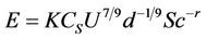
Much of the pioneering work for water evaporation work was performed by Sutton [6]. Sutton proposed the following equation based largely on empirical work:
 (2)
(2)
where Cs is the concentration of the evaporating fluid (mass/volume), U is the wind speed, d is the area of the pool, Sc is the Schmidt number and r is the empirical exponent assigned values from 0 to 2/3. Other parameters are defined as above. The terms in this equation are analogous to the very generic equation (1), proposed above. The turbulence is expressed by a combination of the wind speed, U, and the Schmidt number, Sc. The Schmidt number is the ratio of kinematic viscosity of air (ν) to the molecular diffusivity (D) of the diffusing gas in air, i.e. a dimensionless expression of the molecular diffusivity of the evaporating substance in air. The coefficient of the wind power typifies the turbulence level. The value of 0.78 (7/9) as chosen by Sutton, represents a turbulent wind whereas a coefficient of 0.5 would represent a wind flow that was more laminar. The scale length is represented by d and has been given an empirical exponent of −1/9. This represents, for water, a weak dependence on size. The exponent of the Schmidt number, r, represents the effect of the diffusivity of the particular chemical, and historically was assigned values between 0 and 2/3 [5].
This expression for water evaporation was subsequently used by those working on oil spills to predict and describe oil and petroleum evaporation. Much of the literature follows the work of Mackay [7,8]. Mackay and Matsugu [7] corrected the equations for hydrocarbons using the evaporation rate of cumene. Data on the evaporation of water and cumene have been used to correlate the gas phase mass transfer coefficient as a function of wind-speed and pool size by the equation:
 (3)
(3)
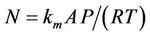
where Km is the mass transfer coefficient in units of mass per unit time and X is the pool diameter or the scale size of evaporating area. Stiver and Mackay [8] subsequently developed this further by adding a second equation:
 (4)
(4)
where N is the evaporative molar flux (mol/s), km is the mass transfer coefficient at the prevailing wind (m/s), A is the area (m2), P is the vapour pressure of the bulk liquid (Pascals), R is the gas constant [8.314 Joules/ (mol-K)], and T is the temperature (K).
Thus, air boundary layer regulation was assumed to be the primary regulation mechanism for oil and petroleum evaporation. This assumption was never tested by experimentation, as revealed by a literature search [2]. The implications of these assumptions are that evaporation rate for a given oil is increased by:
• increasing turbulence
• increasing wind speed, and
• increasing the surface area of a given mass of oil.
These factors can then be verified experimentally to test if oil is boundary-layer regulated or not. These factors formed the basis of experimentation for this paper.
2. Experimental
Evaporation rate was measured by weight loss using an electronic balance. The balance was a Mettler PM4000. The weight was recorded using a laptop computer, a serial cable to the balance and the software program, “Collect” (Labtronics, Richmond, Ontario).
Measurements were conducted in the following fashion. A tared petri dish of defined size was loaded with a measured amount of oil. At the end of the experiment vessels were cleaned and rinsed with dichloromethane and a new experiment started. The weight loss dishes were standard glass petri dishes from Corning. A standard 139 mm diameter (ID) dish was used for most experiments. For the experiments in which area was a variable, dishes of other diameters were employed. Diameters and other dimensions were measured using a Mitutoyo digital vernier caliper. The lip, height of the dish above the oil, with the 139 mm dish varied from 2 to 10 mm depending on depth of fill. For the other dishes the lip varied from 2 to 20 mm.
Measurements were done in one of three locations; inside a fume hood, inside a controlled temperature room, or on a counter top. Some experiments were conducted in the fume hood, where there was no temperature regulation. Temperatures were measured using a Keithley 871 digital thermometer with a thermocouple supplied by the same firm. Temperatures were taken at the beginning and the end of a given experimental run.
The constant temperature chamber (room) employed was a Constant Temperature model. It could maintain temperatures from −40˚C to +60˚C and regulate the chosen temperature within ±1˚C.
In experiments involving wind, air velocities were measured using a Taylor vane anemometer and a Tadi, “Digital Pocket Anemometer”. Measurements were taken at the closest position above the glass vessel floor and at the lip level. These velocities were later confirmed using a hot wire anemometer and appropriate data manipulations of the outputs. The anemometer was a TSI— Thermo Systems model 1053b, with power supply (TSI model 1051-1), averaging circuit (TSI model 1047) and signal linearlizing circuit (TSI model 1052). The voltage from the averaging circuit was read with a Fluke 1053 voltmeter. The hot wire sensor (TSI model 1213-60) was angled at 45˚. The sensor probe resistance at 0˚C was 7.21 ohms and the sensor was operated at 12 ohms for a recommended operating temperature of 250˚C. Data from the hot wire anemometer was collected on a Campbell Scientific CR-10 data logger at a rate of 64 Hz.
Evaporation data were collected on a laptop computer and subsequently transferred to other computers for analysis. The “Collect” program records time and the weight directly. Data were recorded in ASCII format and converted to Excel format. Curve fitting was performed using the software program “TableCurve”, Jandel Scientific Corporation, San Raphael, California.
Oils were taken from supplies of Environment Canada and were supplied by various oil companies for environmental testing. Table 1 lists the properties and descriptions of the test liquids [9].
3. Results and Discussion
Table 2 lists the experiments performed and the results in terms of the best fit equations. These were done by curve fitting using the program Table Curve, as noted above. The best fit was done on the basis of the simplest equation fitting with the highest regression coefficient (R2). The results are presented in the order of the experimental series:
3.1. Wind Experiments
Experiments on the evaporation of oil with and without wind, were conducted with three oils, ASMB (Alberta Sweet Mixed Blend crude oil), Gasoline, FCC Heavy Cycle (a processed oil), and with water. Water formed a baseline data set since much is known about its evaporation behaviour [3,4]. Regressions on the data were performed and the equation parameters calculated, are shown in Table 3. Curve coefficients are the constants

Table 1. Properties of the test liquids.
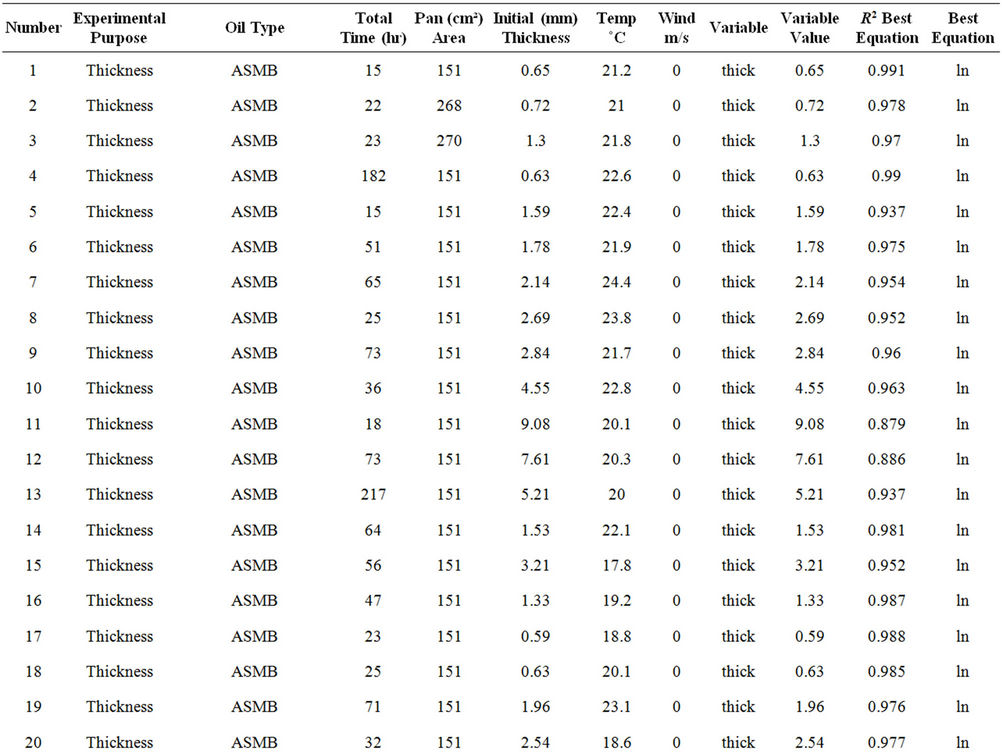
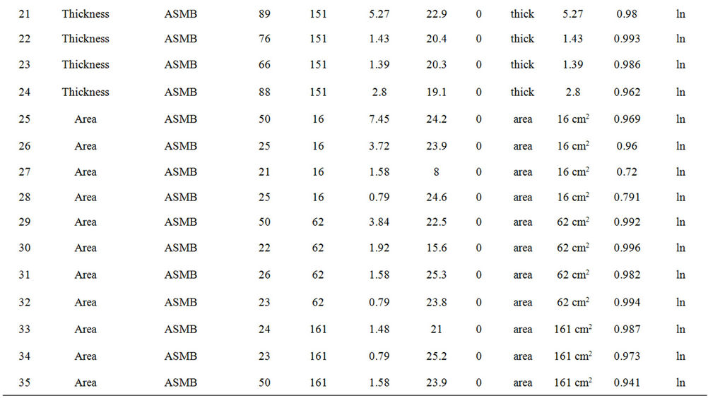

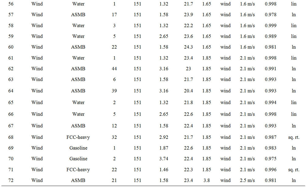
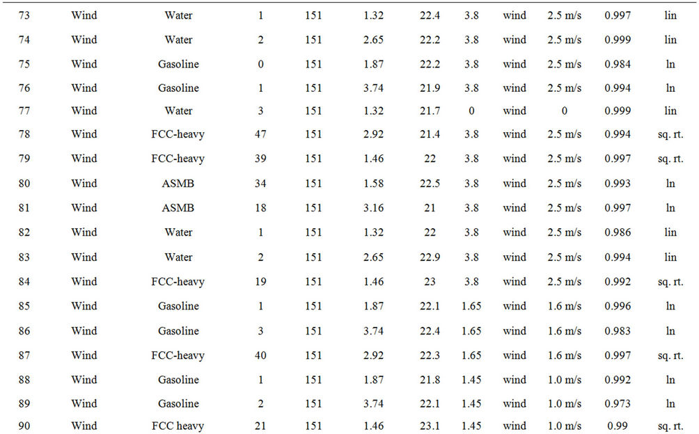
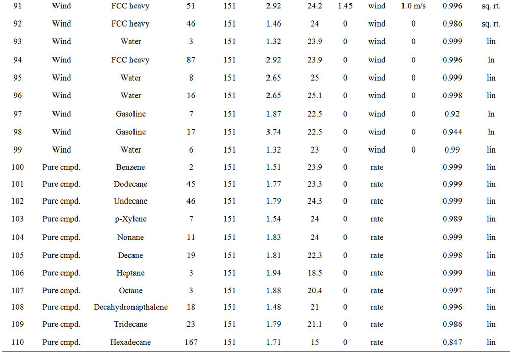
Table 2. Experimental summary.

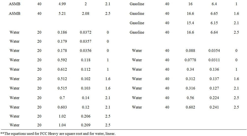
Table 3. Data from the wind tests.
from the best fit equation (Evap = a ln(t), t = time in minutes, for logarithmic equations or Evap = a , for the square root equations). Data were calculated separately for percentage of weight lost and absolute weight. Both values show the small relative upward tendency with respect to wind effects. The plots of wind speed versus the evaporation rate (as a percentage of weight lost) for each oil type are shown in Figures 1 to 4. These figures show that the evaporation rates for oils and even the light products, gasoline and FCC Heavy Cycle, are
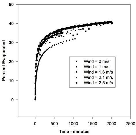
Figure 1. Evaporation of ASMB with varying wind velocities.
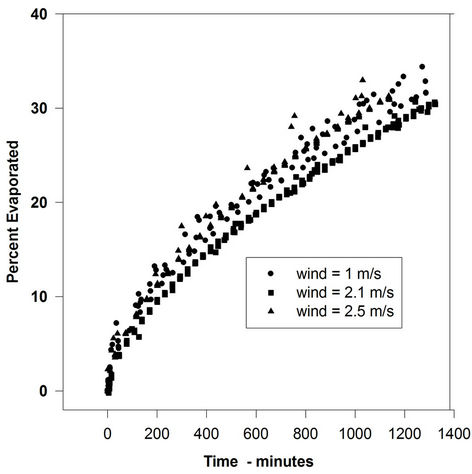
Figure 2. Evaporation of FCC-Heavy with varying wind velocities.
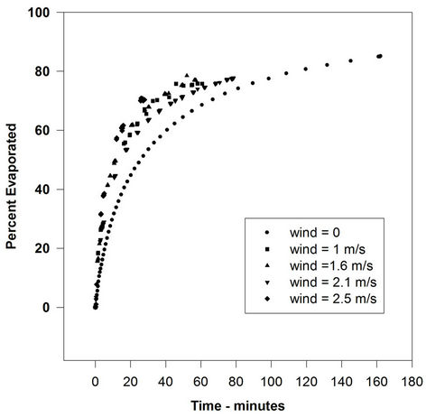
Figure 3. Evaporation of gasoline with varying wind velocities.
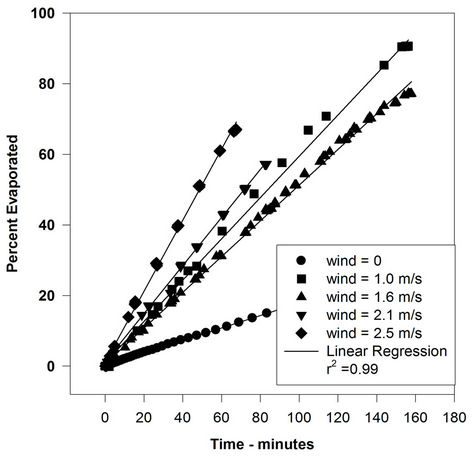
Figure 4. Evaporation of water (20 g) with varying wind velocities.
not increased by a significant amount with increasing wind speed. In some cases, there is a small rise from the 0-wind level to the 1-m/s level, but after that, the rate remains relatively constant. The evaporation rate after the 0-wind value is nearly identical for all oils. The oil evaporation data can be compared to the evaporation of water, as illustrated in Figure 4.
These data show the classical relationship of the water evaporation rate correlated with the wind speed (evaporation varies as U0.78, where U is wind speed). This indicates that the oils used here are not boundary-layer regulated. Figure 5 shows the rates of evaporation compared to the wind speed for all the liquids used in this study. This figure shows the evaporation rates of all test liquids versus wind speed. The lines shown are those calculated by linear regression using the graphics software, SigmaPlot (Washington, DC). This clearly shows that water evaporation rate increased, as expected, with increasing wind velocity. The oils. ASMB, FCC heavy cycle and gasoline, do not show a measurable increase with increasing wind speed. In any case, the oils do not show the U0.78 relationship that water shows.
All the above data show that oil is not boundary-layer regulated. Water shows the classic boundary-layer regulation.
3.2. Study of Mass and Evaporation Rate
ASMB oil was again used to conduct a series of experiments with volume as the major variant. Alternatively thickness and area were held constant to ensure that the strict relationship between these two variables did not affect the final regression results. Figure 6 illustrates the relationship between evaporation rate and volume of evaporation material (also equivalent to mass of evaporating material). This figure illustrates a strong correlation between oil mass (or volume) and evaporation rate. This suggests no air boundary-layer regulation is at work, since for an air boundary-layer regulated material evaporation is not affected by mass in the same area.
3.3. Study of the Evaporation of Pure Hydrocarbons—with and without Wind
A study of the evaporation rate of pure hydrocarbons was

Figure 5. Correlation evaporation rates and wind velocities.
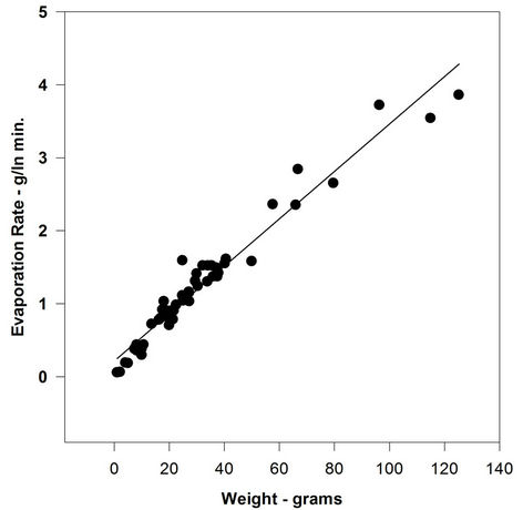
Figure 6. Correlation of mass with evaporation rate.
conducted to test the classic boundary-layer evaporation theory as applied to the hydrocarbon constituents of oils. The evaporation rate data are illustrated in Figure 7. This figure shows that the evaporation rates of the pure hydrocarbons have a variable response to wind. Heptane (hydrocarbon number 7) shows a large difference between evaporation rate in wind and no wind conditions, indicating boundary-layer regulation. Decane (carbon number 10) shows a lesser effect and Hexadecane (carbon number 16) shows a negligible difference between the two experimental conditions. This experiment shows the extent of boundary-regulation and the reason for the small or negligible degree of boundary-regulation shown by crude oils and petroleum products. Crude oil contains very little material with carbon numbers less than decane, often less than 3% of its composition [9]. Even the more volatile petroleum products, gasoline and diesel fuel only have limited amounts of compounds more volatile than decane, and thus are also not strongly boundary-layer regulated.
3.4. Saturation Concentration
Another evaluation of evaporation regulation is that of saturation concentration, the maximum concentration soluble in air. Table 4 lists the saturation concentrations of water and several oil components [10]. This table shows that saturation concentration of water is less than that of many common oil components. The saturation concentration of water is in fact, about two orders less in magnitude than the saturation concentration of volatile oil components such as pentane. This further explains why oil has a air boundary-layer limitation much higher than that of water and thus is not air boundary-layer regulated.
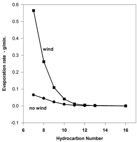
Figure 7. evaporation rates of pure compounds.

Table 4. Saturation concentration of water and hydrocarbons.
4. Conclusions
Oil evaporation is not air boundary-layer regulated. The results of the following experimental series have shown the lack of boundary-layer regulation: 1) a study of the evaporation rate of several oils with increasing wind speed shows that the evaporation rate does not change measurably with wind level. Water, known to be boundary-layer regulated, does show a significant increase with wind speed, U (Ux, where x varies from 0.5 to 0.78, depending on the turbulence level); 2) the volume or mass of oil evaporating correlates with the evaporation rate. This is a strong indicator of the lack of boundary-layer regulation because with water, volume (rather than area) and rate do not correlate; 3) evaporation of pure hydrocarbons with and without wind (turbulence) shows that compounds larger than nonane and decane are not boundary-layer regulated. Most oil and hydrocarbon products consist of compounds larger than these two and thus would not be expected to be boundary-layer regulated.
Having concluded that boundary-layer regulation is not specifically applicable to oil evaporation, it remains to explain why this is so. The reason is twofold: oil evaporation is relatively slow compared to the threshold where it would be air boundary-layer regulated; and the threshold to boundary-layer regulation for oil evaporation is much higher than that for water. These two factors were highlighted two ways:
1) A comparison of the maximum rates of evaporation for some oils, gasoline and water, in the absence of wind, shows that some oil rates exceed that for water by as much as an order of magnitude (water = 0.034 g/min, ASMB = 0.075 g/min, and Gasoline = 0.34 g/min; all under the specific conditions noted), and 2) The saturation concentration of several hydrocarbons in air reveals that some hydrocarbon saturation concentrations in air can be greater than that of water by as much as two orders-of-magnitude.
The fact that oil evaporation is not air boundary-layer regulated implies a simplistic evaporation equation will suffice to describe the process. The following factors do not require consideration: wind velocity, turbulence level, area, and scale size. The factors important to evaporation include time and temperature. Thickness is a factor above certain thicknesses, which are probably not relevant to a rapidly spreading oil slick. The latter is the subject of further experimentation.
REFERENCES
- M. Fingas, “Oil and Petroleum Evaporation,” Proceedings of the 34th Arctic and Marine Oilspill Program Technical Seminar, Vancouver, 4-6 October 2011, pp. 426- 459.
- M. Fingas, “A Literature Review of the Physics and Predictive Modelling of Oil Spill Evaporation,” Journal of Hazardous Materials, Vol. 42, No. 2, 1995, pp. 157-175. doi:10.1016/0304-3894(95)00013-K
- W. Brutsaert, “Evaporation into the Atmosphere,” Reidel Publishing Company, Dordrecht, 1982.
- F. E. Jones, “Evaporation of Water,” Lewis Publishers, Chelsea, 1992.
- J. L. Monteith and M. H. Unsworth, “Principles of Environmental Physics,” Hodder and Stoughton, London, 2008.
- O. G. Sutton, “Wind Structure and Evaporation in a Turbulent Atmosphere,” Proceedings of the Royal Society of London, Vol. 146, No. 858, 1934, pp. 701-722.
- D. Mackay and R. S. Matsugu, “Evaporation Rates of Liquid Hydrocarbon Spills on Land and Water,” The Canadian Journal of Chemical Engineering, Vol. 51, No. 4, 1973, pp. 434-439. doi:10.1002/cjce.5450510407
- W. Stiver and D. Mackay, “Evaporation Rate of Spills of Hydrocarbons and Petroleum Mixtures,” Environmental Science and Technology, Vol. 18, No. 11, 1984, pp. 834- 840. doi:10.1021/es00129a006
- Environment Canada, “Online Catalogue of Crude Oil and Oil Product Properties,” 2011. http://www.etc-cte.ec.gc.ca/databases/OilProperties/oil_prop_e.html
- Z. Wang and M. Fingas, “Oil and Petroleum Product Fingerprinting Analysis by Gas Chromatographic Techniques,” In: L. M. L. Nollet, Ed., Chromatographic Analysis of the Environment, Taylor and Francis, Boca Raton, 2005, pp. 1027-1101.
- “Ullmann’s Encyclopedia,” Ullmann Publishing, Hamburg, 2005-2009.