Journal of Transportation Technologies
Vol.3 No.1(2013), Article ID:27308,20 pages DOI:10.4236/jtts.2013.31008
Forecasting Baltic Dirty Tanker Index by Applying Wavelet Neural Networks
1Logistics and Transport Research Group, Department of Business Administration, School of Business, Economics and Law at University of Gothenburg, Göteborg, Sweden
2Economic Commission for Latin America and the Caribbean (ECLAC), Santiago, Chile 3Transport Research Institute (TRI), Edinburgh Napier University, Edinburgh, UK
Email: gordon.wilmsmeier@cepal.org
Received November 12, 2012; revised December 15, 2012; accepted December 25, 2012
Keywords: BDTI; Tanker Freight Rates; Forecasting; Wavelets; Neural Networks; Shipping Finance
ABSTRACT
Baltic Exchange Dirty Tanker Index (BDTI) is an important assessment index in world dirty tanker shipping industry. Actors in the industry sector can gain numerous benefits from accurate forecasting of the BDTI. However, limitations exist in traditional stochastic and econometric explanation modeling techniques used in freight rate forecasting. At the same time research in shipping index forecasting e.g. BDTI applying artificial intelligent techniques is scarce. This analyses the possibilities to forecast the BDTI by applying Wavelet Neural Networks (WNN). Firstly, the characteristics of traditional and artificial intelligent forecasting techniques are discussed and rationales for choosing WNN are explained. Secondly, the components and features of BDTI will be explicated. After that, the authors delve the determinants and influencing factors behind fluctuations of the BDTI in order to set inputs for WNN forecasting model. The paper examines non-linearity and non-stationary features of the BDTI and elaborates WNN model building procedures. Finally, the comparison of forecasting performance between WNN and ARIMA time series models show that WNN has better forecasting accuracy than traditionally used modeling techniques.
1. Introduction
Research on tanker shipping generally focus on freight rates, fleet arrangements, ship chartering decisions, shipping strategies, operation optimization, etc. [1-6], the freight rate complexity in connection to forecasting techniques is of particular interest in this paper. An inherent feature of shipping freight rates are fluctuations as a source of market risks for all market participants, including not only tanker shipping companies, but also hedge funds, commodity and even energy producers [7]. In essence, forecasting is about attaining and analyzing the right information of the present [cf.8]. Decision makers in the shipping industry often utilize information on historical freight rates to make strategic decisions [cf.8], thus appropriate forecasting techniques may enable the actors in shipping business to make better decisions.
Due to the high volatility in the tanker shipping market accurate prediction of future tanker freight rates is challenging. Currently, the crude oil tanker freight rate freight forward agreements (FFA) are mainly referred to the routes included in the Worldscale [9] and Baltic Dirty Tanker Index [10]. Due to the short history of the BDTI research concerning forecasting of crude oil tanker indexes and rates has only emerged in the last decade. This paper offers new thoughts on the application of hybrid artificial intelligent techniques—Wavelet Neural Networks, beyond traditional modeling and forecasting methods in the shipping sector.
2. Literature Review
Prevailing research determining and forecasting shipping freight rates is based on stochastic and econometric explanation modeling techniques. Stochastic modeling is related to probability theory in the modeling of phenomena in technology and natural sciences. There are numerous examples in bulk and tanker shipping research using stochastic modeling methods. Cullinane [11] firstly developed a short-term adaptive forecasting model for The Baltic International Freight Futures Exchange speculation, through a Box-Jenkins approach, which revolves around what is referred to as ARIMA (p, d, q) modeling. Cullinane measured the predictive power of his model and compared it with alternative forecasting models at that time.
By utilizing Autoregressive Conditional Heteroscedasticity (GARCH) model, Kavussanos [12] determined that smaller size tankers show more flexibility compared to larger tanker ships in terms of their business pricing and operations. Jonnala & Bessler [13] also used GARCH for the specification and estimation of an ocean grain rate equation. Based on sample freight rates data, Veenstra & Franses [14] demonstrated the series of freight rates to be non-stationary, utilizing freight rate data in a vector autoregressive model to forecast dry bulk shipping freight rates. Presenting a stochastic optimal control problem the property of the equilibrium of tanker shipping freight rates is discussed to be close to that of the standard geometric mean reversion process [15]. Adland & Cullinane [5] utilized a general non-parametric Markov diffusion method to investigate the dynamics of tanker spot freight rates, arguing that non-linear stochastic models can best describe these dynamics. However, due to the high volatility in spot freight rates, the difficulties in detecting slow-speed mean reversion in high frequency data became a constraint for the model [5]. Batchelor et al. [10] examined the performance of popular time series models in forecasting spot and forward rates on major seaborne freight routes, and they found the vector equilibrium correction model (VECM), to deliver the best in-samplefit, however, the predictive ability of the VECM in reality is poor. Batchelor et al. [10] suggested ARIMA and VAR model as better models for forecast. Goulielmos & Psifia [16] demonstrated the non-normality and nonlinearity in trip and time charter freight rate indices by using the BDS test, thus arguing that linear and other traditional models are not suitable for modeling the distributions of the indices [16]. Sødal et al. [17] explored the market switching of different ship types based on numerical experiments with a mean-reverting model. They concluded that new combination carriers may enter the market in the near future [17].
The non-linearity, non-stationary and complex inherent characteristics of shipping freight rates make traditional stochastic modeling methods hard to achieve a good balance between forecasting accuracy and theoretical feasibility of the models.
The earliest econometric explanation modeling application in tanker freight rate research can be traced back to 1930s. Koopmans [18] studied the determinants of tanker freight rates by modeling the supply and demand for tanker shipping services. Since that time, numerous tanker freight rate studies have been following Koopmans ideas. Zannetos [19] argued that static expectations in tanker ship supply and demand necessarily imply a future price level equal to current prices, thus the future price level of tanker freight rates under static conditions can be derived from objective data before any changes in present prices occur. Evans [20] analyzed the matching of supply and demand for bulk shipping in the short and long run. Even though initially Evans’ research was not designed for tanker shipping, the use of static models shows is of similar nature to that of Zanneto’s in analyzing the supply and demand in shipping by econometric explanation modeling methods. In contrast to static models, dynamic econometric models emphasize the interrelationship and interactions among the variables. It has been demonstrated that mathematical analysis of dynamic econometric models is a valuable tool for predicting future time tracks of certain economic variables [21]. In tanker shipping freight rate mechanism studies, recent research exerts the stochastic extension of traditional partial shipping supply and demand equilibrium models of the VLCC spot freight market, and simulates the probability distribution of future spot freight rates and fleet size based on present market situations collective with stochastic demand by using a dynamic model [22].
Econometric modeling methods are able to incorporate causality. Econometric explanation modeling methods are widely adopted in the shipping freight rate related research, despite its known limitations. In comparison to stochastic modeling methods, econometric modeling methods are generally less capable in modeling uncertainties. Additionally, even if the rationales or causalities behind the fluctuations in shipping freight rate may be explained by econometric models, in order to model the causalities, bundles of constraints and assumptions about the data and variables are requested by the econometric model, thus the used causalities are often found to be deficient in the modeling process.
Because of the limitations of traditional stochastic and econometric explanation models, the combination of wavelets and neural networks may provide an interesting opportunity. The Wavelet Neural Networks (WNN) concept is based on wavelet transformation theory and was first proposed by Zhang & Benveniste [23], as an alternative to feed forward neural networks for approximating arbitrary nonlinear functions [23]. The main feature of WNN is that it combines the time frequency localization properties and adaptive learning nature of neural networks [24,25], thus making WNN a useful tool for analyzing and forecasting time series, especially when the data series is non-linear and non-stationary.
3. Modeling
3.1. Determinants of BDTI
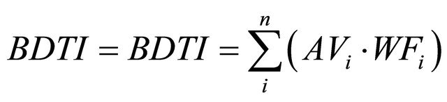
The Baltic Exchange Dirty Tanker Index (BDTI) indicates the cost of shipping unrefined petroleum oil, on a basis of the average costs of 17 routes. The average rate (AVi) of each route is calculated by the Baltic Exchange in cooperation with a panel of major ship broking companies. The panelists calculate weighting factors of each route. The BDTI is defined as the sum of the multiplications of the average rates (AVi) of each route with the weighing factor (WFi) of that particular route. The calculation can be illustrated by the following function:
 [26].
[26].
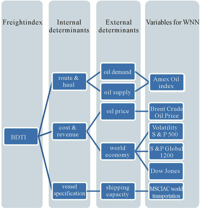
The supply of ships balanced against cargo demand, the balance of fleet capacity and cargo volumes are considered to be the most significant assessment factors and direct indicators for the market [27]. The BDTI is calculated on the basis of its internal determinants, which are route, haul, cost & revenue and vessel specification:
The route: due to changes in the geography and balance of fronthaul and backhaul routes of oil trade only a limited number of trade routes can become the standard routes in the BDTI index. The supply of ships balanced against cargo demand determines routes [27].
Load and discharge ports: The load and/or discharge port may be fixed outside the route definitions the difference between the ports is assessed on the basis of market significance. This normally includes the factors of port costs, extra steaming time or savings and other added value due the geographical difference [27].
Vessel specifications: include deadweight, overall length, draft, capacity, service speed and bunker consumption [27]. Due to economies of scale the average vessel capacity determines patterns and trends of the BDTI.
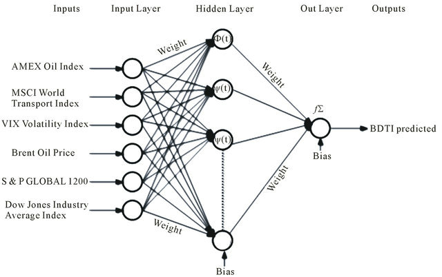
In this paper, the set of internal determinants are extended further by including the external determinants of oil demand, supply price, world economy and fleet capacity. Correspondingly, six indices are introduced to represent the external determinants and applied in the WNN model for forecasting BDTI trends (see Figure 1).
3.2. The Method
A Wavelet is a “small wave”, which grows and decays within a limited time period. A Wavelet is in clearly contrary to “big wave”, which swing up and down for a very long, even infinite time period, for instance, the sine wave is a typical “big wave”
 .
.
By defining a real value function  over a real axis
 , the quantifying notion of a wavelet can be expressed as follows [cf.28]:
 (1)
(1)
 (2)
(2)
Therefore, in a given interval , for any
Source: Authors
Figure 1. Determinants of BDTI.
 , there must be
 (3)
(3)
Equation (2) describes function  having a movement away from zero, while Equation (1) describes that movements above zero must be canceled out by movements below zero. Since the interval
  is utmost small compared to the infinite long real axis
 , the non-zero movement of
  therefore can be regard as limited to a small time interval.
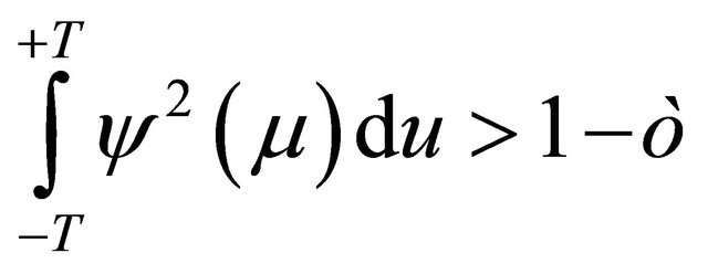
In order to utilize wavelets, the following common additional condition defined as admissibility condition needs to be considered:
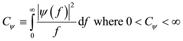 (4)
(4)
Under this condition, a wavelet  is admissible, thus allowing reconstruction of a function from its wavelet transform.
The application of wavelets allows the adapting the representations of data to the nature of the information. Wavelets have many advantages over traditional Fourier analysis methods in analyzing conditions where discontinuities and sharp spikes exist in the signal [29]. Traditional Fourier analysis, which expresses a signal as a sum of a series of sine and cosine (“big waves”), is good for studying stationary data; however, since many changes in a market will happen within a transient time, Fourier analysis is not well suited for studying data with transient events that can be hardly predicted from the historical data [30]. Wavelets fill this gap by the notion of small wave processing, which is designed with a high level of non-stationary data capturing ability.
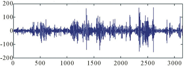
Wavelets are well-suited for approximating data with sharp discontinuities [29]. The BDTI can be regard as a kind of signal, with sharp spikes all along the line (Figure 2).
Using wavelets analysis allows isolating and processing specific types of patterns concealed in the masses of data. Wavelet transformations allow time-frequency localization for the signal or data [30]. This enables to not only capture repeating background signals in the BDTI, but also individual, localized, specific variations in the background. Therefore, the authors use wavelets to approximate BDTI data, thus cutting the data into different frequency components each with its own solution (pattern) matched to its scale, and then process these components with neural networks.
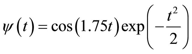
Generally speaking, wavelet analysis explores the signals with short duration and finite energy. Wavelet analysis transforms the signal under investigation into another presentation, which expresses the signal in a more useful pattern [30]. Wavelet analysis procedure adopts a wavelet prototype function, often called, mother wavelet, through temporal analysis, which is performed with a contracted, high-frequency version of the prototype function, and frequency analysis, which is performed using dilated, low-frequency version of the prototype wavelet, so to expand and shift wavelet of varying scales and positions to approximate the original signal or data [28,29]. The Morlet wavelet function  is often referred to as the mother wavelet (6) [cf.31]:
 (6)
(6)
where  s is the scaling parameter,
  is the translation parameter, t is the time, and
  is the basis function of the wavelet
 .
.
For the purpose of this paper, the Morlet wavelet is adopted as the mother wavelet since it offers a good formulation of time frequency methods and a resolution for smoothly changing time series [28,32]. Hence, the Morlet wavelets are used for wavelet transformations and selected as the hidden layer nodes in the future neural network construction.
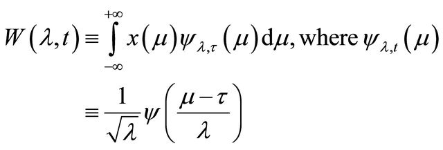
Each element of the wavelet set is a scaled (dilated or compressed) and translated (shifted) Morlet mother wavelet, that can be formulated as follows:
 (7)
(7)
Certain functions of the selected wavelet family can then be presented without any loss of information as a linear combination in the discrete case, or as an integral in the continuous case using wavelet transformation [33].
The wavelet functions constitute the wavelet transformation to analyze the signal in its time, scale, and frequency content [29]. Wavelet transformation can be localized in both time and frequency domains, by using a scaling and translating wavelet function [34]. The continuous wavelet transformation (CWT) and discrete wavelet transformation (DWT) are main classes for different wavelets [28].
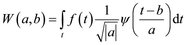
The continuous wavelet transformation is designed to deal with the time series defined over a continuous real axis:
 (8)
(8)
where , .
, . is the function or signal. The idea behind CWT is to calculate the amplitude coefficient thus making
  best fit the signal
 , given
  dilation factor, and
 ![]() translation factor. The adjustments in
translation factor. The adjustments in  enables to see how the wavelet fits the signal from dilation, and changes in
![]() reveal the nature of signal changes over time. CWT preserves all the information from the original data series or signal-
reveal the nature of signal changes over time. CWT preserves all the information from the original data series or signal- . If this
 and signal
  meet the given conditions in Equations (1)-(4), then the wavelet can be reconstructed following inverse transformation:
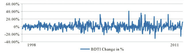
Source: Authors, based on BDTI
Figure 2. BDTI change in percentage, 1998 to 2011.
 (9)
(9)
where  is defined in Equation (4).
Thus, the CWT and signal  represent the same entity in contents, but CWT shows the information in a new manner [28]. Since the Morlet wavelet is a typical continuous wavelet the authors utilize CWT to gain new insights in BDTI data series.
Discrete wavelet transform (DWT) works with time series defined over a specific range of integers [28], and it is the operation that generates a data structure containing  components of a variety of lengths, then filling and transforming data structure into a different data vector of length
  [29].
[29].
As presented in previous section, CWT consists a function of and
and , therefore, leading to a result of over abundant information when analyzed. By implementing DWT, we are able to retain the critical features of CWT and view DWT as a discrete sample of the CWT.
 (10)
(10)
This discrete critical sampling of CWT is obtained through  in which discrete translation and dilation are presented by integers j and k. The substitution can be described as following:
 (11)
(11)
The function of j and k is donated as W(j, k), thus, a critical sampling of CWT defines the resolution of DWT from both the time and frequency perspective [30]. The wavelet coefficients can be found by wavelets that follow the values given by:
 (12)
(12)
After knowing the relationship between CTW and DTW, the discrete wavelet is defined as:
 (13)
(13)
where k and j are integers,  , is the fixed dilation factor,
  is the translation factor and depends on the dilation factor. Then the scaling function is defined as [30]:
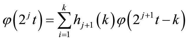 (14)
(14)
The wavelet translation function is defined as:
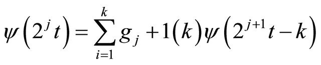 (15)
(15)
So, a signal or a series of data can be expressed as a combination of (14) and (15):
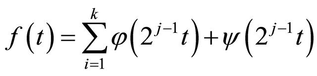 (16)
(16)
The additive decomposition is known as a “multiresolution analysis”, and the generalization of DWT is known as the “wavelet packet” [28]. The process of DWT is achieved by Matlab programming. Therefore, by applying decomposition to the original BDTI series, the sample variance of the original series of BDTI is decomposed based on scale and the amount of redundant information in the data is filtered by this sub-sampling processes.
An example of a 3-layer feed-forward artificial neural network with n inputs, n hidden nodes, and n outputs is illustrated in Figure 3.

Source: Authors.
Figure 3. An example of neural network.
A Neuron is a linear or nonlinear, parameterized, bounded function. The variables of the neuron are called inputs of the neural while its corresponding value is its outputs [35]. The parallel structure of the system means the neurons functions can carry out the computation at the same time. Input layer is not consistent with a fully functional neuron, instead, it is more like a data recorder, which receives the values of a data series from outside the neural networks and then constitutes inputs to next layer. The hidden layer is the processing layer where inputs and outputs remain within neural networks. Output layer sends the output results out of neural networks.
The weights  and parameters are assigned to the inputs
 ![]() of the neurons, thus making a neuron a nonlinear combination of function
of the neurons, thus making a neuron a nonlinear combination of function
 .
.
Bias is an additional constant that is added to the combination of inputs and weights. The most frequently used linear combination v is expressed as a weighted sum of inputs, with bias:
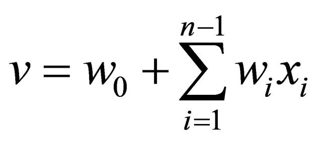 (17)
(17)
The function f is termed as activation function, which is applied to the weighted sum of inputs of a neuron in order to produce the output under a certain threshold, in another words, the activation function manages the amplitudes of the output. Currently, the majority of NN’s use sigmoid functions as activation function such as the tanh function or tangent function as inverse-of the output y of a neuron with inputs ![]() is produced by
is produced by
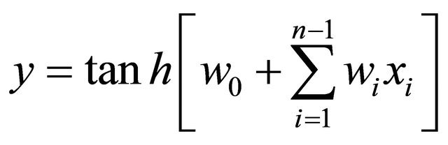 [35].
[35].
The weights are non-linearly assigned to the neurons. The function f to a great extent defines the assigns of weights. For example, the output of Radical Basis Function (RBF) is given by:
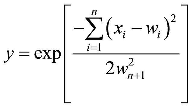 (18)
(18)
where  is weight,
 ![]() is standard deviation.
is standard deviation.
The authors utilize the Morlet wavelet, as the function to assign the weights and to produce the neuron outputs for forecasting. As explained above, a neuron is a nonlinear, and weighted function of its input variables, thus, the neural network is the composition of the nonlinear functions of two or more neurons [35]. Generally, the neural network can be divided into two classes: feedforward neural networks and recurrent/feedback neural networks.
A feedforward neural network is a nonlinear function of its inputs, which is the composition of the functions of its neurons [35]. In this kind of network, only neurons in subsequent layers can be connected, and the information strictly flows from the input layer to the output layer. Each layer receives information only to and from its connected layers. The data processing extends over multiple layers in feedforward direction and no feedback connections exist in the neural network [36].
In a recurrent neural network, there exists at least one path leading back to the neuron. Therefore, in comparison to feedforward neural networks, the recurrent neural network contains feedback connections [37]. Recurrent neural networks are sensitive and can be adapted to the past inputs [38,39]. The recurrent neural network may be effective in this BDTI forecasting research, however, as suggested by Pearlmutter [40], it is more sensible to begin with trying multi-layered feedforward neural networks to solve the problem before applying recurrent neural network [40]. In this paper the authors only utilize feedforward neural networks for forecasting BDTI forecasting.
The weights in the networks are obtained through training. Training is the algorithmic procedure, by which the weights of such a network are estimated, for a given family of functions [35]. The neural network is trained by learning rules then determines suitable weights by itself. Generally, there are two types of learning, supervised and unsupervised learning [41].
This research uses backpropagation, a type of supervised learning that is widely used and a computationally economical method to train neural networks [35,42,43]. Backpropagation is realized by iteratively processing a set of training samples, comparing the outputs of network for each sample with actual known values. The mean square error between real outputs and actual known values is minimized by adjusting the weights for each sample, and this adjust is conducted in a backward direction, from the output layer to the hidden layer [44].
Metrics of backpropagation can be generally described as simple and local nature [45]. Moreover, there are two distinctive advantages of backpropagation training [46]; firstly, it is mathematically calculated to minimize the mean squared aggregate error in all training samples. Secondly, it is a supervised training since the input information vector can be compared with a desired output or target vector. Therefore, it can be implemented on parallel neural networks for BDTI forecasting. Next section elaborates on the aspects of backpropagation training algorithms and WNN.
3.3. The WNN Model
There are two types of WNN. In first type of WNN, input data are merely preliminary treated through the wavelet function, and thus the wavelet and the neural network processing are conducted separately. The second type of WNN replaces the neurons by wavelets, in this situation, weights and thresholds of the neural network are modified by the dilation and translation of wavelets [23]. Theoretically, the three-layer neural networks structure is adequate to solve any arbitrary function approximation [47]. For the BDTI forecasting the latter WNN type is used and a three-layer WNN model is constructed (Figure 4).
In a first step the weights, thresholds of neural network and the dilation and translation parameters of wavelet function are initialized and the dilation parameter as , the translation parameter as
 , neural network connections weights as
 , the learning rate as η, and a momentum factor as
 ![]() and initial values for these parameters are defined. The sampling data calculator set as 1. The learning rate determines how fast the network can learn, that is to say how much the link weights and node biases can be modified based on the change in direction and change rate. A momentum rate allows the network to potentially avoid through local minima.
and initial values for these parameters are defined. The sampling data calculator set as 1. The learning rate determines how fast the network can learn, that is to say how much the link weights and node biases can be modified based on the change in direction and change rate. A momentum rate allows the network to potentially avoid through local minima.
The second step includes training input data and the corresponding expected output , and calculating the outputs of hidden and output layer; where the output of the hidden layer:
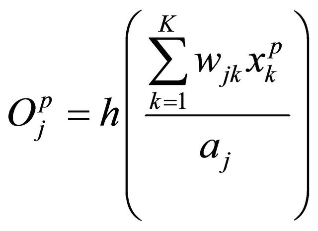 (19)
(19)
and where the output of the output layer:
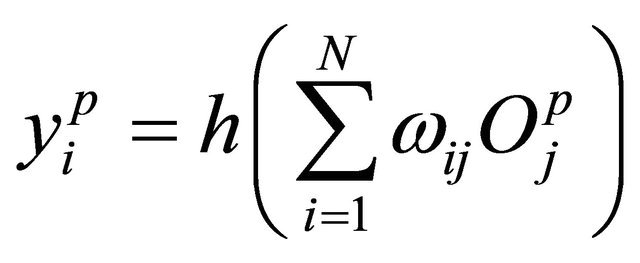 (20)
(20)
In the Equations (19) and (20),  is the input of the output layer,
  is the output of the hidden layer,
 ![]() is the Morlet wavelet (see (6) and (7)).
is the Morlet wavelet (see (6) and (7)).
The third step calculates the error and gradient vectors using the following equations:
 (21)
(21)
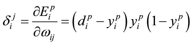 (22)
(22)
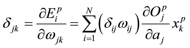 (23)
(23)
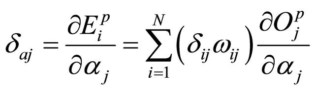 (24)
(24)
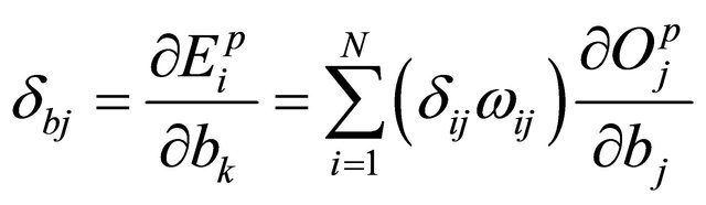 (25)
(25)
In the fourth step the errors will be back propagated through the network, and the weights are adjusted correspondingly as given below:
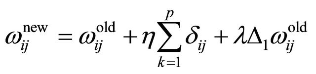 (26)
(26)
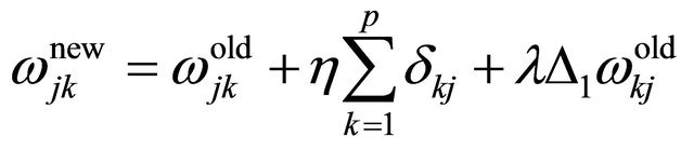 (27)
(27)
Source: Authors.
Figure 4. Forecasting BDTI by WNN Model.
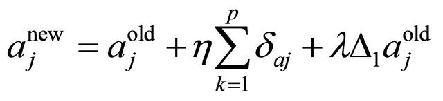 (28)
(28)
 (29)
(29)
The fifth steps inputs the next sample date, so . If the expected error
 , where
 ![]() is the predefined accuracy specification value
is the predefined accuracy specification value , the training of the WNN will be ceased, otherwise, the
 ![]() calculator will be reset to 1 and the training will restart from step 2.
calculator will be reset to 1 and the training will restart from step 2.
3.4. ARIMA Model for Forecasting Comparison
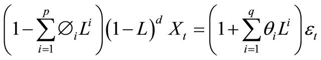
ARIMA (p,d,q) time series is a record of a random variable realized from a stochastic process [48]. The model transforms the non-stationary time series into stationary ones by differencing and logging of original data. In the ARIMA model d, p, q are non-negative integers, and refer to autoregressive terms, non-seasonal differences and moving averages respectively. The mathematic expression of ARIMA is as follows:
An ARIMA (p,q) model is given by:
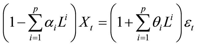 (30)
(30)
where  is the time series data, and t is time. L is the lag operator and
  is the autoregressive term.
  refers to the error term.
If the linear polynomial  has a unitary root of multiplicity d, then
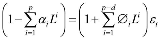
thus an ARIMA (p, d, q) procedure expresses these polynomial factorization characteristics, as given by [49]:
 (31)
(31)
The means absolute error (MAE), root mean square deviation (RMSD) and mean absolute percentage error (MAPE) are used to examine the forecasting accuracy and are defined as:
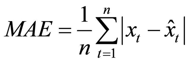 (32)
(32)
where  is the predicted value.
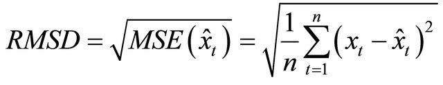 (33)
(33)
 (34)
(34)
4. Modeling Results
4.1. Data
The data includes the daily BDTI value between August 3rd 1998 and February 25th 2011, which is equal to 3147 trading days. The data were supplied by Baltic Exchange London, Ltd.
For the same period, the data of the Brent Oil Price Index, CBOE SPX Volatility Index, and S&P Global 1200 Index were collected from Bloomberg Financial Laboratory; the Amex Oil Index and Dow Jones Industry Average Index data were collected through Yahoo Finance [50], with quotation codes ^XOI and ^DJI.
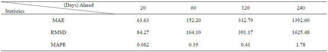
Following Ripley [51], the data is cataloged into three sets: the training set, validation set and test set. The training set refers to a set of example data used for learning, in order to identify the weights. The validation set is a set of examples used to select the number of hidden nodes in a neural network. This set is combined with test data since the hidden nodes will be set through experience. The test set is related to assess the performance of networks. Data sets for 4 weeks (20 days [52]), 12 weeks (60 days), 24 weeks (120 days) and 48 weeks (240 days) are used to examine the performance of WNN and ARIMA.
The data were cleaned in order to make these data valid for the same point in time. The time points of the other six indices data are strictly in line with those of the BDTI, gap values for certain trading days for the six indices are filled using the value of its nearest previous trading day, and redundant values are deleted.
All the data are normalized for WNN to recognize and process them. This is because every Morlet wavelet node’s signal is restricted to a 0 to 1 range and training targets therefore should be normalized between 0 and 1 (see (2), (4), (7), (12) and (15)). The data were normalized as follows:
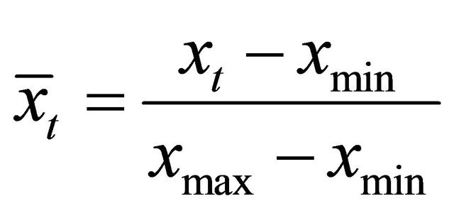 (35)
(35)
4.2. Forecasting BDTI Using ARIMA
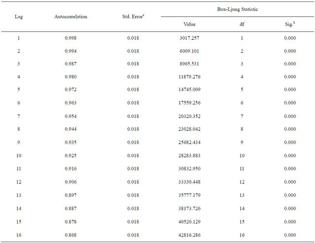
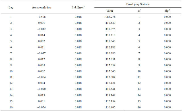
While the WNN has no pre-request in properties of input series data, the ARIMA model can process only stationary series. Therefore, it is necessary to examine whether the BDTI is stationary through auto-correlation analysis using SPSS 19 software.
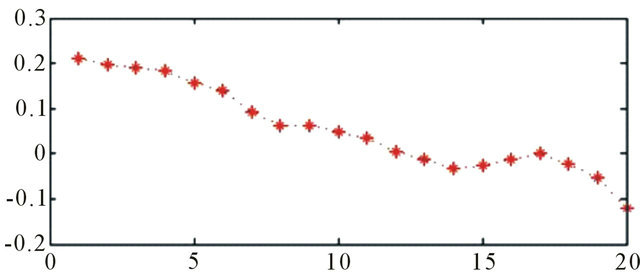
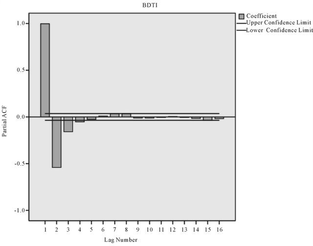
The autocorrelation decreases as the time lag increases (see Appendix, Table A1), confirming that the BDTI series is a non-stationary time series. For ARIMA forecasting, the BDTI data series needs to be transformed into a stationary time series by order difference. The Partial ACF approaches values close to zero after three lags the value of coefficient approaches zero, therefore, the p value is set as 3 (Figure A1).
According to experience, the d, trend value, is usually set by 0, 1, or 2. 0 means no trend exists in the time series. When time series are differenced by one, d = 1, the linear trend is removed. When d = 2, both linear and seasonal trends are removed. Usually, d values of 1 or 2 are adequate to make the mean stationary [48]. Here d is set as 2 for the ARIMA model.
The moving average q is often used to smooth shortterm fluctuations, thus highlighting longer-term trends [48]. According to the BDTI research above, no significant long-term trend has been found, therefore, p is set as 0 for the ARIMA model.
The ARIMA model is set at (3,2,0) for a 120 days forecast, the ARIMA model is only used as a reference model, therefore, the other possible combinations of value (p, d, q) for ARIMA model may be detected by export modeler function of SPSS are ignored.
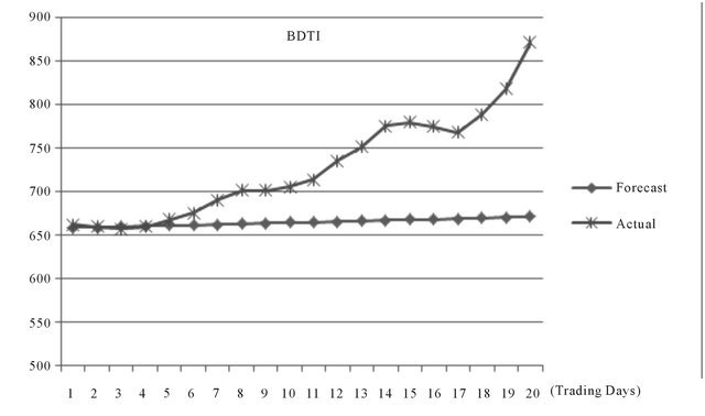
The prediction accuracy of the ARIMA model seems to be acceptable for periods of 40 trading days. The MAPE value is relatively low which means average errors between actual and forecasting values are within ±8% in average (Figure A2, Table 3).
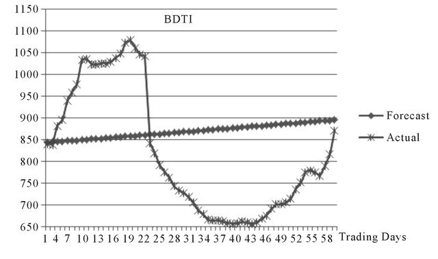
When increasing the forecasting period to 60 days the prediction accuracy of ARIMA model decreases significantly. Given the linear nature of ARIMA, it can hardly catch any fluctuation in this period.
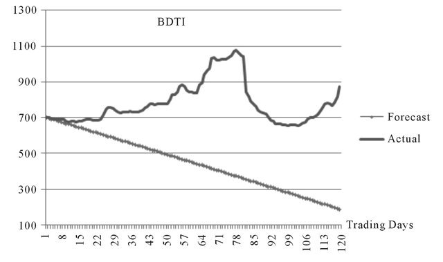
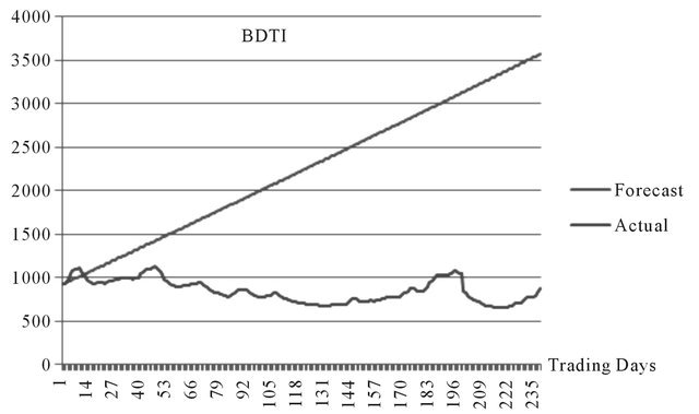
The forecasting results for 120 days are not acceptable, since the errors terms are too significant (Figure A4, Table A3), which indicates the poor forecasting accuracy of ARIMA model in mid or long term (more than three months) non-linear forecast. In Figure A3, it can be observed that ARIMA forecasts a downturn of the BDTI, however, in reality the BDTI experienced a significant increase during that period.
The results for 240 days forecasts (Figure A5, Table A3) reveal the short coming of linear forecasting when forecasting long term non-linear time series.
The results show that the ARIMA model has relatively low predictive accuracy in forecasting BDTI, especially in longer terms. The only acceptable result is for a 20 days ahead forecasting situation, with an 8% average forecasting error, and this result is in line with ElShaarawi & Piegorsch [53].
In addition, the forecasting results by ARIMA are presented in form of linear regression, which can hardly match the non-linear, non-stationary, and volatile nature of BDTI. In 120 and 240 days ahead forecasting, the ARIMA model offers obviously contrary trends of the BDTI contradicting the actual development of the index, the results thus may lead to miserable decision making errors.
4.3. BDTI Forecasting Using WNN
The structure of the WNN model for BDTI forecasting is presented in Figure 4. Six indices are employed that may externally affect the BDTI development, in addition one day BDTI time delay is used as input, to forecast the BDTI. These variables will interact in the “black box” of WNN, and BDTI forecasting value will be used as an output.
The number of hidden notes are assigned by experiences and adjusted according to the time frame of forecasting. The weights are initialed by default random value of the network. The time delay is defined at 1, which means the BDTI index can be influenced by its previous day’s closing value. The learning rate is set at 0.01. The number of iterations for training is defined at a maximum of 800. The margin of error tolerance for training is set at less than 0.001.
Since the WNN forecasting model contains much information, hidden characteristics of the BDTI need to be made more obvious for the six variables to catch. Figuratively speaking, the authors intend to make specific trees become more visible in the forest; therefore, the DWT philosophy and wavelet reconstruction methods are employed. The wavelet transform is used to decompose the time series into varying scales of temporal resolution [54]. The latter provides a sensible decomposition of the data so that the underlying temporal structures of the original time series become more traceable.
The BDTI data is decomposed and then a new BDTI series is reconstructed. The noise and redundant information in the original BDTI data series is filtrated in this process (Figure 5).
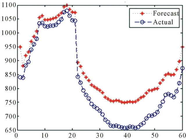
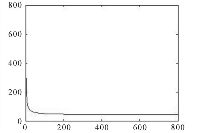
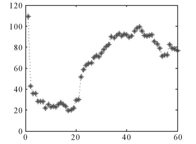
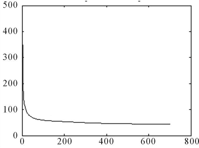
The results of WNN for 20 trading days forecasting show that the WNN model in does not well catch the trend of the actual movement of BDTI (Figure 6). However, the WNN model converges really fast, after around 80 training iterations (Figure A6). The rapid convergence demonstrates the efficiency of wavelet neuron algorisms in neural networks.
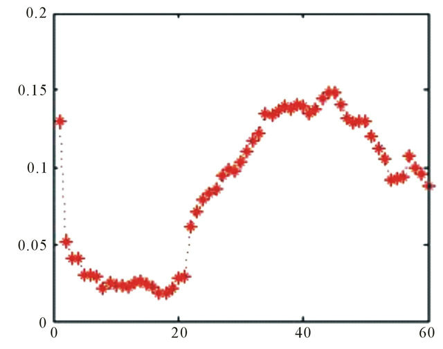
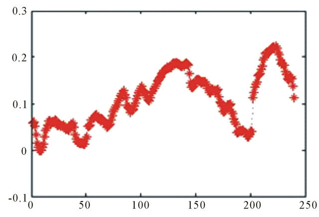
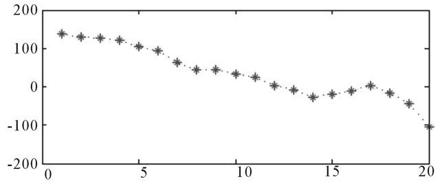
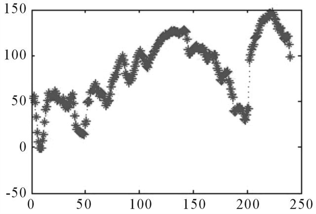
The relative errors indicate the difference between the actual and forecasting values of BDTI. The relative error transforms errors into percentage expressions. The forecasting errors stay within a range of ±100% (Figure A7). The relative error is between 20% and –10% (Figure 7).
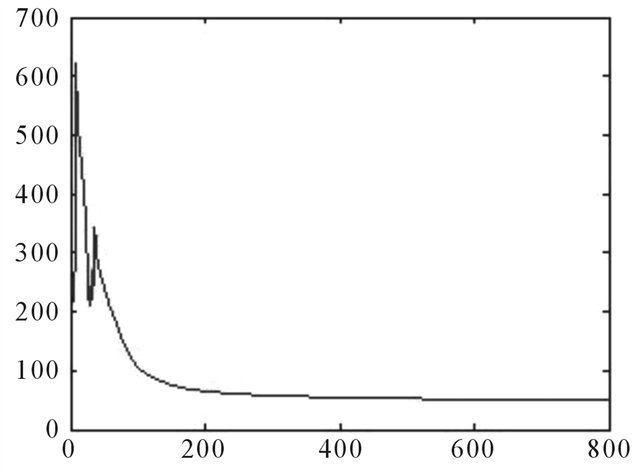
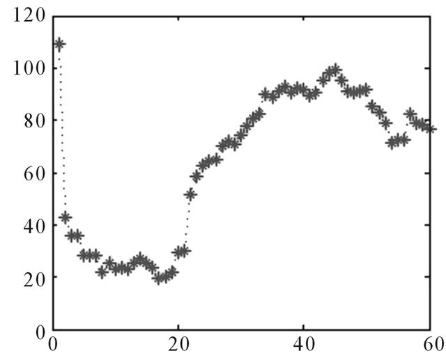
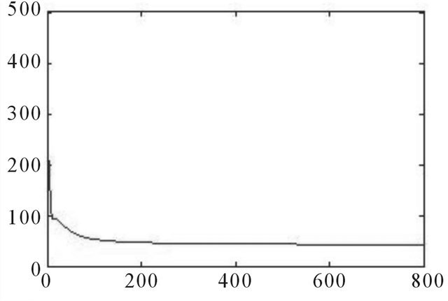
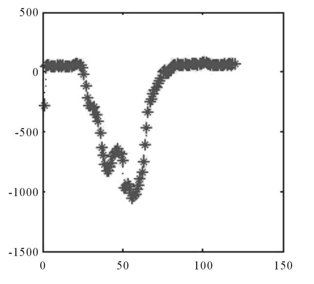
In 60 days ahead forecasting, the WNN captured the upward trend in the first 20 days, but it underestimated the extent of the drop in the BDTI in the following days (Figure 8). The network started to converge after 100 trainings (Figure A8).
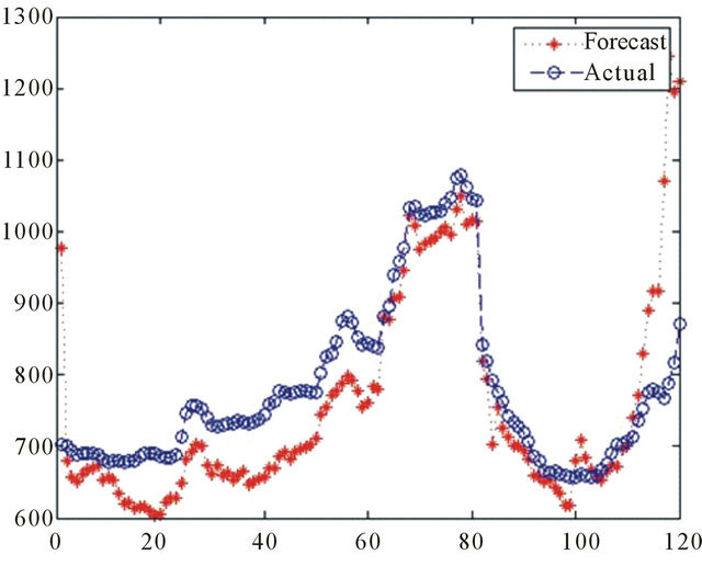
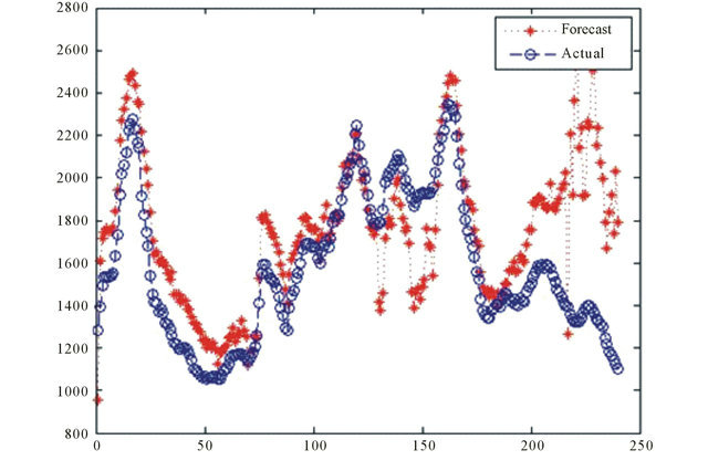
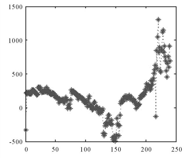
In the 120 days ahead situation the WNN is able to approximate major movements of the BDTI, however, after 110 days, the forecasting values surged much faster than the actual values (Figure 10).
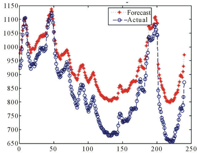
In long term forecasting, the non-linear movements of the BDTI are well approximated by the WNN the model. The WNN model captured the three peaks of the BDTI,
Source: Authors
Figure 5. Filtrated noise—filtrated high frequency components after wavelet reconstruction.

Source: Authors
Figure 6. 20 Days ahead BDTI forecasting by WNN (January 31st 2011-February 25th 2011).
Source: Authors
Figure 7. Relative error, 20 days ahead.
Source: Authors
Figure 8. 60 Days ahead BDTI forecasting by WNN (November 26th 2010-February 25th 2011).
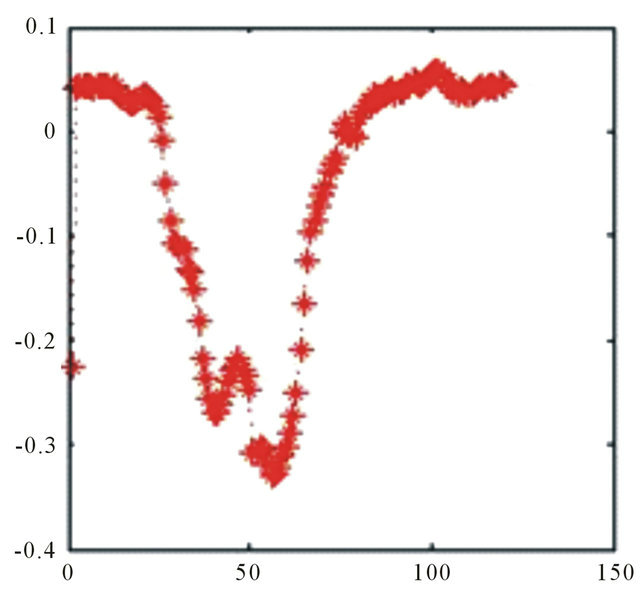
Source: Authors
Figure 9. Relative error, 60 days ahead.
Source: Authors
Figure 10. 120 Days ahead BDTI forecasting by WNN (September 3rd 2010-February 25th 2011).

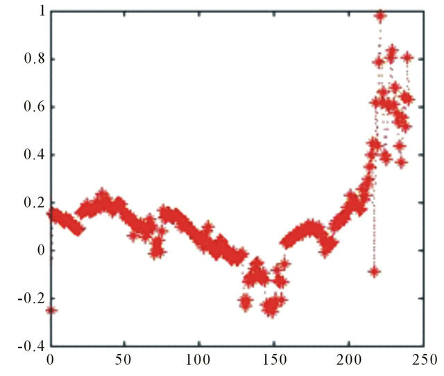
Source: Authors
Figure 11. Relative error, 120 days ahead.
however, it failed to precisely predict the troughs in their full extent (Figure 12).
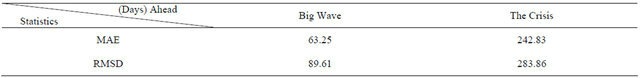
4.4. Forecasting Results of WNN in Challenging Situations
Based on the significant results in comparison to the ARIMA model this section tests the performance of the WNN forecasting model in two very specific and “challenging” time periods, see Figure 14.
In September 2004 to February 2005, BDTI surged to its historical high within three months, and then plummeted in the following three months. Figure 15 shows that the WNN model was able to appropriate the movement of the BDTI during this time period.
Although the WNN model did not adequately predict the climax of BDTI, it provides useful information about the movement trends of BDTI (Figure 16). The current financial crisis started at the end of 2007, and the world economies have still not fully recovered from the crisis. The tanker shipping freight rates and BDTI fluctuated significantly during the global financial crisis.
From Figure 17, it can be seen that the forecasted movements of the BDTI by WNN fluctuated more vocatively than the actual BDTI during this one year time period. The forecasting error maximum can be 100% more than actual value (Figure 18). During the first 100 trading days the WNN presented a relatively good performance, but in later period the WNN seemed to be more sensitive in forecasting, and volatilization became significant.
5. Conclusions
Concluding, there seems to be no significant difference
Source: Authors
Figure 12. 240 days ahead by WNN (March 12th 2010- February 25th 2011).
Source: Authors
Figure 13. Relative error, 120 days ahead.

Source: Authors
Figure 14. BDTI and “challenging situations”.

Source: Authors
Figure 15. “Big wave” forecasting by WNN (September 2004-February 2005).
in performance between WNN and ARIMA model in BDTI short term forecasting. However, for longer periods, the WNN model shows some superiority over ARIMA, offering reasonable non-linear forecasts about the BDTI movements. The forecasting accuracy of WNN decreases as forecasting times increase (Tables A3-A5). Although the WNN model did not perfectly fulfill the forecasting tasks in “challenging situations”, it was able to predict and capture of useful information about trends and movements of the BDTI index.
Source: Authors
Figure 16. Relative error, “big wave”.
Source: Authors
Figure 17. BDTI forecasting during financial crisis (November 2007-November 2008).
Source: Authors
Figure 18. Relative error, “big wave”.
This paper illustrates that artificial intelligent methods can constitute powerful problem solving tools in engineering and natural science, but also have great application potential in shipping research. Traditional stochastic and econometric explanation models are significantly different from machine learning and artificial intelligent methods in nature. Generally, comparing with traditional stochastic and econometric explanation methods, machine learning methods regard to the nature of data mechanism as unknown and complex and allow models to learn from and adapt to their circumstances. Wavelet neural network is a type of hybrid neural network. WNN combines the time frequency localization properties and adaptive learning nature of neural networks thus making it a potential tool for forecasting in complex circumstance.
Examining BDTI forecasting performance, the authors identify that traditional ARIMA forecasting method is weak in forecasting this non-linear and highly fluctuating shipping index, especially for longer time periods. In contrast, the WNN model adopts the artificial intelligent algorisms and combines the wavelet and neural networks, with adequate and appropriate inputs, network design and training, WNN can be a very effective method in forecasting the non-linear and non-stationary shipping index, such as BDTI.
Since WNN can be applied to forecast BDTI, this method can probably also be applied for other analysis of other shipping sectors. WNN offers a good prediction of future trends of the BDTI, which can be used as a relevant tool in market intelligence, business negotiation, decision making and financial budgeting. Shipping companies require rational decision making and market knowledge to optimize their fleet to balance demand and supply in the whole tanker market, which is of particular difficulty and importance in volatile markets.
One short coming in the WNN forecasting model is that the initial weights for neural network are randomly defined by computing software. If the initial weights are far from suitable values, then the network may have to iterate many more times than usual and thus the model may have difficulty in converging. This may lead to poor predicting accuracy and unstable forecast performance. However, this can be partly overcome by applying genetic algorithm optimization methods [55] and/or particle swarm optimization [56] algorithm.
In addition, the number of hidden nodes, training times and lags are assigned according to researcher’s experience. The selection of appropriate number of hidden nodes is a very difficult and tricky task for the design of WNN
REFERENCES
- D. Hawdon, “Tanker Freight Rates in the Short and Long Run,” Applied Economics, Vol. 10, No. 3, 1978, pp. 203- 218. doi:10.1080/758527274
- D. Glen, M. Owen and R. Meer, “Spot and Time Charter Rates for Tankers, 1970-77,” Journal of Transport Economics and Policy, Vol. 15, No. 1, 1981, pp. 45-58
- M. Beenstock and A. Vergottis, “An Econometric Model of the World Tanker Market,” Journal of Transport Economics and Policy, Vol. 23, No. 3, 1989, pp. 263-280.
- A. Perakis and W. Bremer, “An Operational Tanker Scheduling Optimization System: Background, Current Practice and Model Formulation,” Maritime Policy and Management, Vol. 19, No. 3, 1992, pp. 177-187. doi:10.1080/751248659
- R. Adland and K. Cullinane, “The Non-Linear Dynamics of Spot Freight Rates in Tanker Markets,” Transportation Research Part E: Logistics and Transportation Review, Vol. 42, No. 3, 2006, pp. 211-224. doi:10.1016/j.tre.2004.12.001
- R. Laulajainen, “Operative Strategy in Tanker (Dirty) Shipping,” Maritime Policy and Management, Vol. 35, No. 3, 2008, pp. 315-341.
- T. Angelidis and S. G. Skiadopoulos, “Measuring the Market Risk of Freight Rates: A Value-at-Risk Approach,” International Journal of Theoretical and Applied Finance, Vol. 11, No. 5, 2008, pp. 447-469. doi:10.1142/S0219024908004889
- M. Stopford, “Maritime Economics,” 3rd Edition, Routledge, New York, 2009. doi:10.4324/9780203891742
- Worldscale Association, “Introduction to Worldscale Freight Rate Schedules,” 2011. http://www.worldscale.co.uk/company%5Ccompany.htm
- R. Batchelor, A. Alizadeh and I. Visvikis, “Forecasting Spot and Forward Prices in the International Freight Market,” International Journal of Forecasting, Vol. 23, No. 1, 2007, pp. 107-114.
- K. Cullinane, “A Short-Term Adaptive Forecasting Model for BIFFEX Speculation: A Box—Jenkins Approach,” Maritime Policy and Management: The Flagship Journal of International Shipping and Port Research, Vol. 19, No. 2, 1992, pp. 91-114.
- M. Kavussanos, “Price Risk Modelling of Different Sized Vessels in Tanker Industry Using Autoregressive Conditional Heteroscedasticity GARCH Models,” Transportation Research Part E: Logistics and Transportation Review, Vol. 32, No. 2, 1996, pp. 161-176.
- F. Jonnala, S. Fuller and D. Bessler, “A GARCH Approach to Modelling Ocean Grain Freight Rates,” International Journal of Maritime Economics, Vol. 4, No. 2, 2002, pp. 103-125. doi:10.1057/palgrave.ijme.9100039
- A. W. Veenstra and P. H. Franses, “A Co-Integration Approach to Forecasting Freight Rates in the Dry Bulk Shipping Sector,” Transportation Research Part A: Policy & Practice, Vol. 31, No. 6, 1997, pp. 447-458.
- J. Tvedt, “Shipping Market Models and the Specification of Freight Rate Processes,” Maritime Economics and Logistics, Vol. 5, No. 4, 2003, pp. 327-346. doi:10.1057/palgrave.mel.9100085
- A. M. Goulielmos and M. Psifia, “A Study of Trip and Time Charter Freight Rate Indices: 1968-2003,” Maritime Policy and Management, Vol. 34, No. 1, 2007, pp. 55-67. doi:10.1080/03088830601103418
- S. Sødal, S. Koekebakkera and R. Adland, “Market Switching in Shipping—A Real Option Model Applied to the Valuation of Combination Carriers,” Review of Financial Economics, Vol. 17, No. 3, 2008, pp. 183-203. doi:10.1016/j.rfe.2007.04.001
- T. Koopmans, “Tanker Freight Rates and Tankship Building,” The Economic Journal, Vol. 49, No. 196, 1939, pp. 760-762. doi:10.2307/2225041
- Z. S. Zannetos, “The Theory of Oil Tankship Rates: An Economic Analysis of Tankship Operations,” MIT— Massachusetts Institute of Technology, Cambridge, 1964, pp. 60-64.
- J. J. Evans, “An Analysis of Efficiency of the Bulk Shipping Markets,” Maritime Policy and Management: The Flagship Journal of International Shipping and Port Research, Vol. 21, No. 4, 1994, pp. 311-329.
- S. Reutlinger, “Analysis of a Dynamic Model, with Particular Emphasis on Long-Run Projections,” Journal of Farm Economics, Vol. 48, No. 1, 1966, pp. 88-106. doi:10.2307/1236181
- R. Adland and S. P. Strandenes, “A Discrete-Time Stochastic Partial Equilibrium Model of the Spot Freight Market,” Journal of Transport Economics and Policy (JTEP), Vol. 41, No. 2, 2007, pp. 189-218.
- Q. Zhang and A. Benveniste, “Wavelet Networks,” IEEE Transactions on Neural Networks, Vol. 3, No. 6, 1992, pp. 889-898. doi:10.1109/72.165591
- Z. Wang and Y. Tan, “Research of Wavelet Neural Network Based Host Intrusion Detection Systems,” Proceedings of the International Computer Conference 2006 on Wavelet Active, Chongqing, 29-31 August 2006, pp 1007-1012.
- K. K. Minu, M. C. Lineesh and C. J. John, “Wavelet Neural Networks for Nonlinear Time Series Analysis,” Applied Mathematical Sciences, Vol. 4, No. 50, 2010, pp. 2485-2495.
- K. G. Goulias, “Transport Science and Technology,” Elsevier Ltd., Amsterdam, 2007.
- The Baltic Exchange, “Manual for Panelists—A Guide to Freight Reporting and Index Production,” Unpublished Manuscript, The Baltic Exchange, London, 2011.
- D. B. Percival and A. T. Walden “Wavelet Methods for Time Series Analysis,” Cambridge University Press, Cambridge, 2006.
- A. Graps, “An Introduction to Wavelets,” IEEE Computational Sciences and Engineering, Vol. 2, No. 2, 1995, pp. 50-61. doi:10.1109/99.388960
- K. P. Soman, K. I. Ramachandran and N. G. Resmi, “Insight into Wavelets,” 3rd Edition, PHI Learning Pvt. Ltd., Coimbatore, 2010.
- L. Debnath, “Wavelet Transforms and Their Applications,” Springer, Boston, 2002. doi:10.1007/978-1-4612-0097-0
- J. Lewalle, “Wavelets without Lemmas on Applications of Continuous Waveletsto Data Analysis,” Syracuse University, Syracuse, 1998. http://www.ecs.syr.edu/faculty/lewalle/papers/vki1.pdf
- D. Veitch, “Wavelet Neural Networks and Their Application in the Study of Dynamical Systems,” Networks, Vol. 1, No. 8, 2005, pp. 313-320.
- I. Daubechies, “The Wavelet Transform, Time-frequency Localization and Signal Analysis,” IEEE Transactions on Information Theory Society, Vol. 36, No. 5, 1990, pp. 961-1005. doi:10.1109/18.57199
- G. Dreyfus, “Neural Networks: Methodology and Applications,” Springer-Verlag, Berlin, Heidelberg, New York, 2005.
- A. Abraham, “Artificial Neural Networks. Handbook of Measuring System Design,” John Wiley and Sons Ltd., Hoboken, 2005.
- D. P. Mandic and J. A. Chambers, “Recurrent Neural Networks for Prediction: Learning, Algorithms, Architectures and Stability,” John Wiley and Sons Ltd., Hoboken, 2001. doi:10.1002/047084535X
- M. Casey, “The Dynamics of Discrete-Time Computation, with Application to Recurrent Neural Networks and Finite State Machine Extraction,” Neural Computation, Vol. 8, No. 6, 1996, pp. 1135-1178. doi:10.1162/neco.1996.8.6.1135
- G. Dematos, M. S. Boyd, B. Kermanshahi, N. Kohzadi and I. Kaastra, “Feedforward versus Recurrent Neural Networks for Forecasting Monthly Japanese Yen Exchange Rates,” Asia-Pacific Financial Markets, Vol. 3, No. 1, 1996, pp. 59-75.
- B. A. Pearlmutter, “Dynamic Recurrent Neural Networks,” School of Computer Science Carnegie Mellon University, Defense Advanced Research Projects Agency, Information Science and Technology Office, 1990. http://www.bcl.hamilton.ie/~barak/papers/CMU-CS-90-196.pdf
- K. Cannons and V. Cheung, “An Introduction to Neural Networks,” Iowa State University, Ames, 2002. http://www2.econ.iastate.edu/tesfatsi/NeuralNetworks.CheungCannonNotes.pdf
- R. Hecht-Nielsen, “Theory of the Backpropagation Neural Network,” International Joint Conference on Neural Networks (IJCNN), Vol. 1, Washington DC, 18-22 June 1989, pp. 593-605.
- P. J. Werbos, “Backpropagation Through Time: What It Does and How To Do It,” Proceedings of the IEEE, Vol. 78, No. 10, 1990, pp. 1550-1560. doi:10.1109/5.58337
- J. Han and M. Kamber, “Data Mining: Concepts and Techniques,” Morgan Kaufmann, San Francisco, 2006.
- T. Hastie, R. Tibshirani and J. Friedman, “The Elements of Statistical Learning: Data Mining, Inference, and Prediction,” Springer, New York, 2009.
- P. K. Simpson, “Neural Networks Theory, Technology, and Applications, Institute of Electrical and Electronics Engineers, Technical Activities Board,” University of Michigan, Ann Arbor, 1996.
- R. M. Golden, “Mathematical Methods for Neural Network Analysis and Design,” The MIT Press, Cambridge, 1996.
- K. M. Vu, “The ARIMA and VARIMA Time Series: Their Modelings, Analyses and Applications,” AuLac Technologies Inc., Ottawa, 2007.
- T. C. Mills, “Time Series Techniques for Economists,” Cambridge University Press, Cambridge, 1990.
- Yahoo, “Get Quotes, Historical Prices,” 2012. http://finance.yahoo.com/
- B. D. Ripley, “Pattern Recognition and Neural Networks,” Cambridge University Press, Cambridge, 1996.
- The 20 trading days is based on the following assumption: 1 week = 5 trading days, 1 month = 4 week.
- A. H. El-Shaarawi and W. W. Piegorsch, “Encyclopedia of Environmetrics,” Wiley, Hoboken, 2002.
- A. Aussem and F. Murtagh, “Combining Neural Network Forecasts on Wavelet-Transformed Time Series,” Connection Science, Vol. 9, No. 1, 1997, pp. 113-122. doi:10.1080/095400997116766
- J. J. Merelo, M. Patón, A. Cañas, A. Prieto and F. Morán, “Optimization of a Competitive Learning Neural Network by Genetic Algorithms,” New Trends in Neural Computation, Vol. 686, 1993, pp. 185-192. doi:10.1007/3-540-56798-4_145
- J. Kennedy and R. Eberhart, “Particle Swarm Optimization,” Proceedings of IEEE International Conference on Neural Networks, Vol. 4, Perth, 27 November-1 December 1995, pp. 1942-1948. doi:10.1109/ICNN.1995.488968
Appendix (Figures)
Source: Authors.
Figure A1. Partial ACF of BDTI.
Source: Authors.
Figure A2. 20 days ahead by ARIMA.
Source: Authors.
Figure A3. 60 days ahead by ARIMA.
Source Authors.
Figure A4. 120 days ahead by ARIMA.
Source: Authors.
Figure A5. 240 days ahead by ARIMA.
Source: Authors.
Figure A6. Error changes with training times—convergence speed, 20 days ahead.
Source: Authors.
Figure A7. Errors, 20 days ahead.
Source: Authors.
Figure A8. Error changes with training times—convergence speed, 60 days ahead.
Source: Authors.
Figure A9. Errors, 60 days ahead.
Source: Authors.
Figure A10. Error changes with training times—convergence speed, 120 days ahead.
Source: Authors.
Figure A11. Errors, 120 days ahead.
Source: Authors.
Figure A12. Error changes with training times—convergence speed, 240 days ahead.
Source: Authors.
Figure A13. Errors, 240 days ahead.
Source: Authors.
Figure A14. Errors, “big wave”.
Source: Authors.
Figure A15. Errors, “the crisis”.
Appendix (Tables)
Table A1. Autocorrelations of BDTI series.
Source: Authors Table A2. Autocorrelations of BDTI after 3 differences.
Source: Authors Table A3. BDTI forecasting performance statistics of ARIMA.
Source: Authors Table A4. BDTI forecasting performance statistics of WNN.

Source: Authors Table A5. BDTI forecasting performance statistics of WNN, in challenging situations.
Source: Authors