ABSTRACT

Environmental systems including our atmosphere oceans, biological… etc. can be modeled by mathematical equations to estimate their states. These equations can be solved with numerical methods. Initial and boundary conditions are needed for such of these numerical methods. Predication and simulations for different case studies are major sources for the great importance of these models. Satellite data from different wide ranges of sensors provide observations that indicate system state. So both numerical models and satellite data provide estimation of system states, and between the different estimations it is required the best estimate for system state. Assimilation of observations in numerical weather models with data assimilation techniques provide an improved estimate of system states. In this work, highlights on the mathematical perspective for data assimilation methods are introduced. Least square estimation techniques are introduced because it is considered the basic mathematical building block for data assimilation methods. Stochastic version of least square is included to handle the error in both model and observation. Then the three and four dimensional variational assimilation 3dvar and 4dvar respectively will be handled. Kalman filters and its derivatives Extended, (KF, EKF, ENKF) and hybrid filters are introduced.

Keywords:

Least Square Method, Data Assimilation, Ensemble Filter, Hybrid Filters

1. Introduction

In general, models could be classified as [1] [2] :

1) Process specific models (Causality Process) are based on conservation of laws of nature e.g.: Shallow water modeling, Navier Stokes Equation.

2) Data specific models (correlation based) are based on developed experimental models e.g.: Time Series models, Machine Learning, Neural Networks. etc.

Atmospheric and oceans models are process specific models which Navier stokes equations are the core of the solver to predict, simulate and estimate system states. Process specific models have different classifications from different perspectives, time, space, and structure of the model, in addition to another classification which is deterministic and stochastic.

It is assumed that the state of dynamical system evolves according to first order nonlinear equation

$X_{K+1}=M\left(X_K\right)$ (1)

where $X_K$ is the current state of the system; M(.) is the mapping function from the Current state X at time K to the next state X at K + 1

・ If the mapping function M(.) doesn’t depend on the time index K then it is called a time invariant or autonomous system

・ If the M(.) varies with time index k that is $X_{K+1}=M_K\left(X_k\right)$ , then it is called time-varying system (dynamic system)

・ If $X_{K+1}=M{X}_K$ for M non-singular matrix, then it is called time invariant linear system.

・ If matrix M varies with time, that is $X_{K+1}=M_K{X}_k$ , then it is called time varying linear or non-autonomous system.

・ In the special cases when M(.) is an identity map, that is $M\left(x\right)=x$ , then it is called static system

The mentioned above is the deterministic case; the Randomness in the model can enter in three ways:

(A) Random initial conditions (B) Random forcing (C) Random Coefficients

So, a random or a stochastic model is given by:

$X_{K+1}=M\left(X_K\right)+W_{K+1}$ (2)

where the random sequences $\left\{W_K\right\}$ , denotes to the external forcing; typically $\left\{W_K\right\}$ captures uncertainties in the model including model error.

So, the classes of models that are used in the data assimilation could be classified as:

(1) Deterministic-Static (3) Stochastic-Static

(2) Deterministic-Dynamic (4) Stochastic-Dynamic

The paper is organized as follow: Section 2 states the mathematical foundation for data assimilations which describes linear and nonlinear least square in addition to weighted least square and Recursive Least square. Section 3 introduces the deterministic static model linear and nonlinear cases. Section 4 shows stochastic static model: Both linear and nonlinear cases. Section 5 describes deterministic dynamic linear case and the recursive case. Section 6 explains stochastic dynamic linear, nonlinear, reduced and hybrid filters.

2. Mathematical Background

Mainly all the data assimilation techniques are based on least square estimation, so classification of the estimation problems based on different criteria. The Estimation problems can be underdetermined problem when number of observations (m) are less than number of state (n) (m < n). And can be over determined when number of observations (m) is larger than number of states (n) (m > n) [1] . Also the Estimation problem can be classified according to the mapping function from the state space to observation space which can be linear or nonlinear. and nonlinearity should be handled

Other type of classification is offline or online problems. Where offline problems if the observations are known priori. In other words we have historical set of data and we treat with them. While Online/Sequential problems are computing a new estimate of the unknown state X as a function of the latest estimate and the current observation. So, online formulation is most useful in real time applications. The last type of classifications is Strong and Weak Constraints, The Strong Constraint is occurred when the estimation is performed under the perfect model assumption. While in case of allowing for errors in the model dynamics, it is considered Weak Constraint [1]

Since, Data Assimilation based on Least Square Approach [1] [2] [3] [4] . First we introduce linear version of least square then will move to nonlinear version. After that weighted version for both linear and nonlinear will be introduced.

2.1. Linear Least Square Method

Let $Z=HX$ (3)

Given the observation vector Z and the mapping function/Interpolation matrix H (Full Rank) find the unknown state vector X.

Then the error Vector which represents the difference between the Observations Z and the required estimated state X can be represented as follow

$e=Z–HX$ (4)

The Previous term is called also error term or Innovation term. So we need to find the best estimate that minimizes the error. So the problem is converted from Estimation Problem to Optimization Problem. One of the basic classifications for problem is over determined Problem (m > n) or under determined problem (m < n) and we consider first over determined case (m > n). To measure The vector e using The Euclidean norm and the fact of Minimization of norm is equal to minimization of square norm. The cost function will be as follow

$J\left(x\right)={\Vert Z-HX\Vert }_2^2={\left(Z-HX\right)}^{\text{T}}\left(Z-HX\right)$ (5)

And minimization of X is Obtained under the following condition $\nabla J\left(x\right)=0$ . This lead to

$X={\left(H^{\text{T}}H\right)}^{-1}{H}^{\text{T}}Z$ (6)

And this equation was known as normal equation method. In case of over determined problem m > n. While in case under determined case (m < n). The estimation for X will be as follow.

$X=H^{\text{T}}{\left(H{H}^{\text{T}}\right)}^{-1}Z$ (7)

And this undetermined problem where m number of observation is less than n, number of unknowns is known in geophysical (physical process physical properties of the earth and its surrounding space Environment) because of the cost of collection of the observation is high. And in case uniquely determined case (m = n) which mean that the error e is zero. The estimated state vector X will be

$X=H^{-1}Z$ (8)

As we can see from the above three formulation that minimization for the cost function ends to Solving system of linear equation, and solving the linear system (A = Xb) of equations can be done using:

o Direct methods (Cholesky decomposition, Q-R decomposition, Singular Value decomposition, …) [5] .

o Iterative methods (Jacobi Method, Gauss-Seidel Method, Successive Over-Relaxation method, …) [5] .

2.2. Non Linear Least Square Method

The problem here will be: Given set of observation Z and knowing the function form h which is nonlinear function. Find the state vector X as shown

$Z=h\left(X\right)$ (9)

And the Innovation term will be

$e=Z-h\left(X\right)$ (10)

And the cost function will be

$J\left(X\right)={\Vert Z-h\left(X\right)\Vert }_2^2={\left(Z-h\left(X\right)\right)}^{\text{T}}\left(Z-h\left(X\right)\right)$ (11)

And so that, the idea here is extension for the linear case by replacing the nonlinear term h(x) with its Linear approximation of Taylor series expansion around an Operating Point let it $X_c$ and in this case it is called first order approximation for nonlinear least square as follow

$h\left(X\right)=h\left(X_c\right)+D_h\left(X_c\right)\left(X-X_c\right)$ (12)

where $D_h\left(X_c\right)$ is the Jacobin matrix of h which is an $m\times n$ matrix given by:

$D_h\left(X_c\right)=\nabla h\left(X_c\right)=\left[\frac{\partial h_i}{\partial X_j}\right]\text{where}1\le i\le m;1\le j\le n$ . (13)

And by substitution of first order approximation of Taylor series expansion in the cost function and giving it name $Q_1\left(x\right)$ and the index one refer for first order

$\begin{array}{c}{Q}_1\left(x\right)=J\left(X\right)={\Vert Z-h\left(X\right)\Vert }_2^2\\ ={\left(z-h\left(X\right)-D_h\left(X_c\right)\left(X–X_c\right)\right)}^{\text{T}}\left(z-h\left(X\right)-D_h\left(X_c\right)\left(X–X_c\right)\right)\end{array}$ (14)

And simplifying the notation by define $g\left(X\right)=\left(Z–h\left(X\right)\right)$

$\begin{array}{c}{Q}_1\left(x\right)=J\left(X\right)={\Vert Z-h\left(X\right)\Vert }_2^2\\ ={\left(g\left(x\right)-D_h\left(X_c\right)\left(X-X_c\right)\right)}^{\text{T}}\left(g\left(x\right)-D_h\left(X_c\right)\left(X-X_c\right)\right)\end{array}$ (15)

And by comparing the previous equation by the linear version.

$J\left(x\right)={\Vert Z-HX\Vert }_2^2={\left(Z-HX\right)}^{\text{T}}\left(Z-HX\right)$ (16)

You will find that every Z was replaced by g(x) and every H is replaced by $D_h\left(X_c\right)$ also every X is replaced by $\left(X-X_c\right)$

And if the gradient is $\nabla Q_1=0$ ; we will obtain

$X-X_c={\left[D_h^{\text{T}}\left(X_c\right)D_h^{\text{T}}\left(X_c\right)\right]}^{-1}\left[D_h^{\text{T}}\left(X_c\right)g\left(X_c\right)\right]$ (17)

And this is iterative approach and given an initial value for $X_c$ and solving the above equation using direct methods or iterative methods then iterate again until $X-X_c$ < prescribed threshold

And by similarity the second order algorithm for non Linear Least Square will be same steps except that Taylor series expansion will be full Quadratic approximation

$h\left(X\right)=h\left(X_c\right)+D_h\left(X_c\right)\left(X-X_c\right)+\frac{1}{2}{D}_h^2\left(X_c\right){\left(\left(X_c\right)\left(X-X_c\right)\right)}^2$ (18)

where the $D_h^2\left(X_c\right)={\nabla }^{2}h\left(X\right)$ is the hussian of $h\left(X\right)$ and by substituting this second order expansion in the nonlinear cost function and giving it name $Q_2\left(x\right)$ since the index 2 refer to second order approximation and Putting the gradient $\nabla Q_2=0$ equal zero you will get the following

$X-X_c={\left[D_h^{\text{T}}\left(X_c\right)D_h^{\text{T}}\left(X_c\right)+g\left(X_c\right){\nabla }^{2}h\left(X\right)\right]}^{-1}\left[D_h^{\text{T}}\left(X_c\right)g\left(X_c\right)\right]$ (19)

And this is iterative approach and given an initial value for $X_c$ and solving the above equation using direct methods or iterative methods then iterate again until $X-X_c$ < prescribed threshold. All the above methods were for deterministic least square where

$Z=HX$ or $Z=h\left(X\right)$ (20)

2.3. The Weighted Least Square Method

If there additive random noise was V presented. Which mean the observation is noisy with as follow

$Z=HX+V$ or $Z=h\left(X\right)+V$ (21)

・ Mean E(V) = zero which mean that the instrument is well calibrated Unbiased and If it is ≠ zero which mean that there is bias (for example under or over reading).

・ Covariance $Cov\left(V\right)=R$ , The covariance matrix for the instrument. which it is property for the instrumentation.

So, for the linear form of Least Square, the cost function will be for linear form will be

$J\left(x\right)={\Vert Z-HX\Vert }_{R^{-1}}^2={\left(Z-HX\right)}^{\text{T}}{R}^{-1}\left(Z-HX\right)$ (22)

And the non Linear form

$J\left(x\right)={\Vert Z-HX\Vert }_{R^{-1}}^2={\left(Z-h\left(X\right)\right)}^{\text{T}}{R}^{-1}\left(Z-h\left(X\right)\right)$ (23)

Also by the same methodology that used above, the best estimate form for Stochastic linear least square after equality for the Gradient to zero will be

$X={\left(H^{\text{T}}{R}^{-1}H\right)}^{-1}{H}^{\text{T}}{R}^{-1}Z$ (24)

And for the stochastic nonlinear least square first order approximation will be

$X-X_c={\left[D_h^{\text{T}}\left(X_c\right)R^{-1}{D}_h^{\text{T}}\left(X_c\right)\right]}^{-1}\left[D_h^{\text{T}}\left(X_c\right)R^{-1}g\left(X_c\right)\right]$ (25)

And for the stochastic nonlinear least square Second order approximation will be

$X-X_c={\left[D_h^{\text{T}}\left(X_c\right)R^{-1}{D}_h^{\text{T}}\left(X_c\right)+b\left(X_c\right){\nabla }^{2}h\left(X_c\right)\right]}^{-1}\left[D_h^{\text{T}}\left(X_c\right)R^{-1}g\left(X_c\right)\right]$ (26)

where $R^{-1}g\left(X_c\right)=b\left(X_c\right)$ for simiplyifing the notation.

2.4. The Recursive Least Square Estimation Approach (Offline/Online Approach)

All the above analysis was assumed that the number m of observations is fixed. which mean by another term it is offline version of least square. So if we don’t know number observation m and they are arrive sequentially in time. There’re two ways to add this new observations:

・ The first approach is to solve the system of linear equation repeatedly after arrival of every new observation. But this approach is very expensive from Computational point of view

・ The second approach is to formulate the following problem which is based on Knowing the Optimal estimate $X^{*}\left(m\right)$ based on the m observations. we need to compute $X^{*}\left(m+1\right)$ based on $m+1$ observation. In more clear words we need to calculate to reach to formulation that can compute the new estimate function of the old estimate plus sequantional term. And this approach is called situational or recursive framework

It was known as mentioned above that the optimal linear least square estimate for $Z=HX$ is $X^{*}\left(m\right)={\left(H^{\text{T}}H\right)}^{-1}{H}^{\text{T}}Z$ . Let $Z_{m+1}$ be the new observation then the $Z=HX$ can be expanded in the form of matrix-vector relation as:

$\left[\begin{array}{c}Z\\ Z_{m+1}\end{array}\right]=\left[\begin{array}{c}H\\ h_{m+1}^{\text{T}}\end{array}\right]X$ (27)

So, the Innovation will be:

$e_{m+1}\left(X\right)=\left[\begin{array}{c}Z\\ Z_{m+1}\end{array}\right]-\left[\begin{array}{c}Z\\ Z_{m+1}\end{array}\right]X$ (28)

So, the Cost function will be:

$J\left(X\right)=e_{m+1}^{\text{T}}{e}_{m+1}$ (29)

$J\left(X\right)={\left(Z-HX\right)}^{\text{T}}\left(Z-HX\right)+{\left(Z_{m+1}-h_{m+1}^{\text{T}}X\right)}^{\text{T}}\left(Z_{m+1}-h_{m+1}^{\text{T}}X\right)$ (30)

So, by taking the gradient and equal it to zero $\nabla J\left(x\right)=0$ . We can get the following

$X^{*}\left(m+1\right)=X^{*}\left(m\right)+K_{m+1}{h}_{m+1}\left[Z_{m+1}-h_{m+1}^{\text{T}}{X}^{*}\left(m\right)\right]$ (31)

where

$K_m=H^{\text{T}}H,K_{m+1}=K_m+h_{m+1}{h}_{m+1}^{\text{T}}$ (32)

The cost of computation for the second term of this equation is less than solving the all system again.

The basic building block for understanding the Data assimilation based on Least Square approach was introduced.

3. Deterministic-Static Models

In Atmospheric science, when we want to assimilate observation data to the model at time step, Two source of information are available, one of them after mapping the observation Z to X and the other source is the Prior information.

The Linear/Non Linear Case

The formulation for the problem, we need the best estimate for X given the two source of information

・ The first source is the given the Observation Z and mapping function H, where the innovation term was $e=Z-h\left(X\right)$

・ The Second source is given the Prior or Background information $X_B$ where the innovation term is $e=X-X_B$

So the cost function for this case will

$J\left(X\right)=J_B\left(X\right)+J_o(X)$ (33)

For linear Case $h(.)=H$

$J\left(X\right)=\frac{1}{2}{\left(X-X_B\right)}^{\text{T}}\left(X-X_B\right)+\frac{1}{2}{\left(Z-HX\right)}^{\text{T}}\left(Z–HX\right)$ (34)

For Nonlinear case $h(.)=h\left(X\right)$

$J\left(X\right)=\frac{1}{2}{\left(X-X_B\right)}^{\text{T}}\left(X-X_B\right)+\frac{1}{2}{\left(Z-h\left(X\right)\right)}^{\text{T}}\left(Z-h\left(X\right)\right)$ (35)

4. Stochastic-Static Models

The formulation for the problem will be the same as in Deterministic/Static problem, we need the best estimate for X given the two source of information

・ The first source is the given the Observation Z and mapping function H, where the innovation term was $e=Z-h\left(X\right)$ and the observation has noise with its covariance R

・ The Second source is given the Prior or Background information $X_B$ where the innovation term is $e=X-X_B$ , and the Background has its Covariance B

So the cost function for this case will

$J\left(X\right)=J_B\left(X\right)+J_o\left(X\right)$ (36)

For linear Case: $h(.)=H$

$J\left(X\right)=\frac{1}{2}{\left(X-X_B\right)}^{\text{T}}{B}^{-1}\left(X-X_B\right)+\frac{1}{2}{\left(Z-HX\right)}^{\text{T}}{R}^{-1}\left(Z-HX\right)$ (37)

For Nonlinear case: $h(.)=h\left(X\right)$

$J\left(X\right)=\frac{1}{2}{\left(X-X_B\right)}^{\text{T}}{B}^{-1}\left(X-X_B\right)+\frac{1}{2}{\left(Z-h\left(X\right)\right)}^{\text{T}}{R}^{-1}\left(Z-h\left(X\right)\right)$ (38)

5. Deterministic-Dynamic

The Dynamical models can be classified as:

where $X_K$ is the state of the dynamical system, so if $X_O$ the initial condition is known, so computing the $X_K$ is a forward problem

It is assumed that $X_O$ is not known. And Estimating $X_O$ based on noisy indirect information is the inverse problem that it is required to solve.

The observations also can be classified as:

And assume the $V_K$ is White noise, has zero mean and Known covariance matrix R, which depend on the nature and the type of instruments used

So, formulation for statement of problem is: given set of noisy observations and the model equations, it is required to estimate the initial

Condition $X_O$ that give best fit between the background states and noisy observations

To conclude there are four different types of problems:

1) Linear Model-Linear observation

2) Linear model-non Linear observation

3) Nonlinear model-linear observation

4) Non linear model-Non linear observation

We will consider only one case only the which is the simplest formulation with both model and observations are linear and the other cases could be checked in [1] [2] .

The Definition of the cost function which is weighted sum of the squared errors is given as:

For linear case

$J\left(X\right)=\frac{1}{2}{\displaystyle {\sum }_{i=1}^N{\left(Z_{Ki}-H{X}_{Ki}\right)}^{\text{T}}{R}^{-1}\left(Z_{Ki}-H{X}_{Ki}\right)}$ (41)

For nonlinear case

$J\left(X\right)=\frac{1}{2}{\displaystyle {\sum }_{i=1}^N{\left(Z_{Ki}-h\left(X_{Ki}\right)\right)}^{\text{T}}{R}^{-1}\left(Z_{Ki}-h\left(X_{Ki}\right)\right)}$ (42)

Depend on the whether the observations are linear or not linear. And the goal is to minimize the J(X) w.r.t $X_o$

In case there background will be included for linear case

$J\left(X\right)=\frac{1}{2}{\left(X-X_B\right)}^{\text{T}}{B}^{-1}\left(X-X_B\right)+\frac{1}{2}{\displaystyle {\sum }_{i=1}^N{\left(Z_{Ki}-H{X}_{Ki}\right)}^{\text{T}}{R}^{-1}\left(Z_{Ki}-H{X}_{Ki}\right)}$ (43)

And for nonlinear case

$J\left(X\right)=\frac{1}{2}{\left(X-X_B\right)}^{\text{T}}{B}^{-1}\left(X-X_B\right)+\frac{1}{2}{\displaystyle {\sum }_{i=1}^N{\left(Z_{Ki}-h\left(X_{Ki}\right)\right)}^{\text{T}}{R}^{-1}\left(Z_{Ki}-h\left(X_{Ki}\right)\right)}$ (44)

There are two approaches for minimization of this cost functions

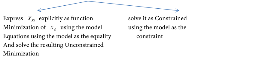
5.1. Deterministic-Dynamic Linear Case

5.1.1. Linear Case-Method of Elimination

This method is mainly based on substitute the following equation $X_K=M_K{X}_o$ in the cost function J(X) then, get the following equation

$J\left(X_o\right)=\frac{1}{2}{\displaystyle {\sum }_{i=1}^N{\left(Z_{Ki}-H{M}_K{X}_o\right)}^{\text{T}}{R}^{-1}\left(Z_{Ki}-H{M}_K{X}_o\right)}$ (45)

Then we get the gradient for the $\nabla J\left(X_o\right)=0$

For simplicity

$J\left(X_o\right)=\frac{1}{2}{X}_o^{\text{T}}A{X}_o-b^{\text{T}}{X}_o+C$ and it is quadratic in $X_o$ (46)

$A={\displaystyle {\sum }_{i=1}^N{M}_K^{\text{T}}{H}^{\text{T}}{R}^{-1}H{M}_K}$ (46-a)

$b={\displaystyle {\sum }_{i=1}^N{M}_K^{\text{T}}{H}^{\text{T}}{R}^{-1}{Z}_K}$ (46-b)

$C=\frac{1}{2}{\displaystyle {\sum }_{i=1}^N{M}_K^{\text{T}}{R}^{-1}{Z}_K}$ (46-c)

So, the gradient is $\nabla J\left(X_o\right)=A{X}_o-b=0$ which leads to

$X_o=A^{-1}b$ (47)

But, this approach is not practical, since it involves matrix-matrix products in the computation of A and b, so there is need to another way

5.1.2. Linear Case-Lagrangian Multipliers Formulation

Define Lagrangian L:

$\begin{array}{l}L\left(X_o,\lambda \right)=\frac{1}{2}\underset{\_}{{\displaystyle {\sum }_{i=1}^N{\left(Z_K-H{X}_K\right)}^{\text{T}}{R}^{-1}\left(Z_K-H{X}_K\right)}}+{\displaystyle {\sum }_{i=1}^N{\lambda }_K^{\text{T}}\underset{\_}{\left(X_K-M{X}_{K-1}\right)}}\\ \text{Objective}\text{function}\text{Model}\end{array}$ (48)

And the Necessary conditions for the minimum

${\nabla }_{X_o}L=0$ (49-a)

${\nabla }_{X_K}L=0$ (49-b)

${\nabla }_{{\lambda }_K}L=0$ (49-c)

So ${\nabla }_{{\lambda }_K}L=0\to X_K-M{X}_{K-1}=0\to X_K=M{X}_{K-1}$ (50-a)

${\nabla }_{X_K}L=0\to H^{\text{T}}{R}^{-1}\left[H{X}_K-Z_K\right]+{\lambda }_K-M^{\text{T}}{\lambda }_{K+1}=0$ (50-b)

${\nabla }_{X_N}L=0\to H^{\text{T}}{R}^{-1}\left[H{X}_N-Z_N\right]+{\lambda }_N=0$ (50-c)

Defining:

$f_K=H^{\text{T}}{R}^{-1}\left[Z_K-H{X}_K\right]=\text{normalizedforecasterrorviewedfrommodelspace}$ (51)

And substitute it in the last two equations

$-f_K+{\lambda }_K-M^T{\lambda }_{K+1}=0\to {\lambda }_K=M^{\text{T}}{\lambda }_{K+1}+f_K$ (52-a)

$-f_N+{\lambda }_N=0\to {\lambda }_N=f_N$ (52-b)

So, as shown that the formulation for calculate $\lambda$ is backword relation. we can iterate backward starting from ${\lambda }_N$ to Compute ${\lambda }_1$ . And this technique is known as backword adjoint dynamics. Then after getting ${\lambda }_1$ substitute in ${\nabla }_{X_o}J\left(X_o\right)=-M^{\text{T}}{\lambda }_1$ and get the gradient then use any minimization algorithm to get $X_o$ , The 4-D Var Algorithm (First order adjoint method) can be summarized as follow:

1) Start with an arbitrary $X_o$ , and compute the model solution using $X_{K+1}=M{X}_K$

2) Given the observation $\left\{Z_K\right\}$ where $1\le K\le N$

3) Set → ${\lambda }_N=f_N$ and Solve ${\lambda }_K=M^{\text{T}}{\lambda }_{K+1}+f_K$ to find ${\lambda }_1$

4) Compute the gradient ${\nabla }_{X_o}J\left(X_o\right)=-M^{\text{T}}{\lambda }_1$

5) Use this gradient in minimization algorithm to find the optimal $X_o$ by repeating the steps 1 through 4 until convergence.

5.2. Recursive Least Squares Formulation of 4D Var (Online Approach)

In the previous part of 4Dvar section the solution for off-line 4Dvar problem of assimilating given set of observations in deterministic-dynamic model using classical least square method.

Now there is need to develop an online or recursive method for computing the estimate of the state as new observations arrive. which mean we need to compute the $X_{N+1}$ in terms of $X_N$ and the new observation $Z_{N+1}$ .

Consider linear deterministic dynamical system without model noise

$X_{K+1}=M{X}_K$ (53)

where the initial condition $X_o$ is random variable with $E\left(X_o\right)=m_o$ and $Cov\left(X_o\right)=P_o$ . and the observations $Z_K$ for $K=1,2,3,\cdots$ are given as

$Z_K=H_K{X}_K+V_K$ (54)

where $H_K$ is full rank and $V_K$ is the observation vector noise with the following known properties

$E\left(V_k\right)=0$ and $Cov\left(V_K\right)=R_K$ (55)

So, the objective function that

$J_N=J_N^P+J_N^o$ (56)

where

$J_N^P=\frac{1}{2}{\left(m_o-X_o\right)}^{\text{T}}{P}_o^{-1}\left(m_o-X_o\right)$ (57)

$J_N^o=\frac{1}{2}{\displaystyle {\sum }_{K=1}^N{\left(Z_K-H_K{X}_K\right)}^{\text{T}}{R}_K^{-1}\left(Z_K-H_K{X}_K\right)}$ (58)

Since, our goal to find an optimal $X_N$ that minimize the $J_N$ , it is needed to express $m_o$ and $X_K$

In tem of the corresponding N values $X_N$ and $m_N$ . So,

Since, $X_N=M_{N-1}{M}_{N-2}\cdots M_K{X}_K=M\left(N-1:K\right)X_K$ (59)

Then $X_K=M^{-1}\left(N-1:K\right)X_N=B\left(N-1:K\right)X_N$ (60)

Since $m_{K+1}=M_K{m}_K=M\left(K:0\right)m_o$ (61)

Hence, the trajectory of the model starting from $m_o=B\left(N-1:0\right)m_N$

Substitute for $X_K$ and $m_o$ into $J_N$

$\begin{array}{c}{J}_N\left(X_N\right)=\frac{1}{2}{\left(m_N-X_N\right)}^{\text{T}}\left[B^{\text{T}}\left(N-1:0\right)P_0^{-1}B\left(N-1:0\right)\right]\left(m_N-X_N\right)\\ +\frac{1}{2}{\displaystyle {\sum }_{K=1}^N{\left(Z_K-H_{K}B\left(N-1:K\right)X_N\right)}^{\text{T}}{R}_K^{-1}\left(Z_K-H_{K}B\left(N-1:K\right)X_N\right)}\end{array}$ (62)

And differentiate $J_N\left(X_N\right)$ w.r.t $X_N$ twice to get the gradient and Hessian. Then setting the gradient to zero and simplifying the notation

$\left(F_N^p+F_N^o\right)X_N=\left(f_N^p+f_N^o\right)$ (63)

where

$F_N^p=B^{\text{T}}\left(N-1:0\right)P_0^{-1}B\left(N-1:0\right)$ (64)

$F_N^o={\displaystyle {\sum }_{K=1}^N{B}^{\text{T}}\left(N-1:K\right)H_K^{\text{T}}{R}_K^{-1}{H}_{K}B\left(N-1:K\right)}$ (65)

$f_N^p=F_N^p{m}_N$ (66)

$f_N^o={\displaystyle {\sum }_{K=1}^N{B}^{\text{T}}\left(N-1:K\right)H_K^{\text{T}}{R}_K^{-1}{Z}_K}$ (67)

By induction the minimization for $X_{N+1}$ of $J_{N+1}\left(X_{N+1}\right)$ is given by

$\left(F_{N+1}^p+F_{N+1}^o\right)X_{N+1}=\left(f_{N+1}^p+f_{N+1}^o\right)$ (68)

The goal of the recursive framework is to express $X_{N+1}$ as function of $X_N$ and $Z_{K+1}$ . this calls when expressing $F_{N+1}^p$ , $F_{N+1}^o$ , $f_{N+1}^p$ , $f_{N+1}^o$ in terms of $F_N^p$ , $F_N^o$ , $f_N^p$ , $f_N^o.$

So using equations from (61) to (64) and $B_K=M_K^{-1}$ and the following equation

$M\left(j:i\right)=\{\begin{array}{l}{M}_j{M}_{j-1},\cdots ,M_{I+1}{M}_I\text{if}j\ge i\\ \text{if}j\ge i\end{array}$ (69)

Then N + 1 formula in terms of N can be get

$F_{N+1}^p+F_{N+1}^o=B_N^{\text{T}}\left[F_N^p+F_N^o\right]B_N+H_{N+1}^{\text{T}}{R}_{N+1}^{-1}{H}_{N+1}$ (70)

$f_{N+1}^p+f_{N+1}^o=B_N^{\text{T}}{F}_N^p{B}_N{m}_{N+1}+B_N^{\text{T}}{f}_N^o+H_{N+1}^{\text{T}}{R}_{N+1}^{-1}{Z}_{N+1}$ (71)

And since

${\left(P_{N+1}\right)}^{-1}=F_{N+1}^p+F_{N+1}^o$ (72)

${\left(P_N\right)}^{-1}=F_N^p+F_N^o$ (73)

$B_N{m}_{N+1}=B_N{M}_N{m}_N=m_N$ (74)

$X_{N+1}^f=M_N{X}_N$ or $X_N=B_N{X}_{N+1}^f$ (75)

$f_{N+1}^p+f_{N+1}^o=B_N^{\text{T}}{\left(P_N\right)}^{-1}{B}_N{X}_{N+1}^f+H_{N+1}^{\text{T}}{R}_{N+1}^{-1}{Z}_{N+1}$ (76)

By combining Equations (70) and (76) into Equation (68) and defining ${\left(P_{N+1}^f\right)}^{-1}=B_N^{\text{T}}{\left(P_N\right)}^{-1}{B}_N$ after combination

$X_{N+1}={\left[{\left(P_{N+1}^f\right)}^{-1}+H_{N+1}^{\text{T}}{R}_{N+1}^{-1}H\right]}^{-1}\left[{\left(P_{N+1}^f\right)}^{-1}{X}_{N+1}^f+H_{N+1}^{\text{T}}{R}_{N+1}^{-1}{Z}_{N+1}\right]$ (77)

The right hand side of this equation is sum of two terms the first one is

${\left[{\left(P_{N+1}^f\right)}^{-1}+H_{N+1}^{\text{T}}{R}_{N+1}^{-1}{H}_{N+1}\right]}^{-1}\left[{\left(P_{N+1}^f\right)}^{-1}{X}_{N+1}^f\right]$ (78)

So adding and subtracting $H_{N+1}^{\text{T}}$ $R_{N+1}^{-1}$ $H_{N+1}$ $X_{N+1}^f$ this term is equal to

$\begin{array}{l}{\left[{\left(P_{N+1}^f\right)}^{-1}+H_{N+1}^{\text{T}}{R}_{N+1}^{-1}{H}_{N+1}\right]}^{-1}\left[{\left(P_{N+1}^f\right)}^{-1}+H_{N+1}^{\text{T}}{R}_{N+1}^{-1}{H}_{N+1}-H_{N+1}^{\text{T}}{R}_{N+1}^{-1}{H}_{N+1}\right]X_{N+1}^f\\ =X_{N+1}^f-K_{N+1}{H}_{N+1}{X}_{N+1}^f\end{array}$ (79)

where

$K_{N+1}={\left[{\left(P_{N+1}^f\right)}^{-1}+H_{N+1}^{\text{T}}{R}_{N+1}^{-1}{H}_{N+1}\right]}^{-1}{H}_{N+1}^{\text{T}}{R}_{N+1}^{-1}$ is called kalman gain matrix and

combine it with Equation (77). The desired recursive expression will be gained

$X_{N+1}=X_{N+1}^f+K_{N+1}\left[Z_{N+1}–H_{N+1}{X}_{N+1}^f\right]$ (80)

6. Stochastic-Dynamic Model

This type of data assimilation problems is same as deterministic/dynamic problems, except that, this type introduces an additional term in the forecast equation which is noise vector that associated with the model (i.e. model error).

For Stochastic-dynamic model we can divide the filters to Linear and Nonlinear filters Linear filter has evolution function $M(.)$ in the model and the mapping function $h(.)$ is linear while in Nonlinear filters those two functions are nonlinear

6.1. Linear Filters

Kalman Linear Filter

Kalman filter approach was first introduced at reference [6] [7]

Problem formulation:

This section will show how model and observation with error will be presented then will formulate the algorithm:

A1-Dynamic model: it will be assumed linear, non autonomous, dynamical system that evolves according to

$X_{K+1}=M_K{X}_K+w_{K+1}$ (81)

where $M_K$ is nonsingular system matrix that varies with time K and $w_K$ denote to model error. It is assumed that $X_o$ and $w_K$ satisfy the following conditions (A) $X_o$ is random variable with known mean vector $E\left(X_o\right)=m_o$ and known covariance matrix $E\left[\left(X_o-m_o\right){\left(X_o-m_o\right)}^{\text{T}}\right]=P_o$ (B) The model erro is unbiased, mean $E\left(w_K\right)=0$ for all k, and temporally uncorrelated (white noise) $E\left(w_K{w}_j^{\text{T}}\right)=Q_K$ when if $j=k$ and $E\left(w_K{w}_j^{\text{T}}\right)=0$ otherwise (C) The model error $w_K$ and the initial state is uncorrelated $E\left(w_K{X}_o^{\text{T}}\right)=0$ for all k

B1-Observations: The observation $Z_K$ is the observation at time k and related to $X_K$ via

$Z_K=H_K{X}_K+V_K$ (82)

where $H_K$ represent the time varying measurement system and $V_K$ represent the measurement noise with the following properties (A) $V_K$ has mean zero $E\left(V_K\right)=0$ (B) $V_K$ is temporary uncorrelated: $E\left(V_K{V}_j^{\text{T}}\right)=R_K$ if $j=k$ while otherwise $E\left(V_K{V}_j^{\text{T}}\right)=0$ . (C) $V_K$ is uncorrelated with the initial state $X_o$ and the model error $w_K$ which mean $E\left(X_o{V}_K^{\text{T}}\right)=0$ for all $K>0$ and $E\left(V_K{W}_j^{\text{T}}\right)=0$ for all K and j

C1-statement of the filtering problem: Given that $X_K$ evolves according to equation 81 and set of observations. Our goal to find an estimate $X_K$ that minimize the mean square error

And the following is the summary of the Kalman filter procedure (Covariance Form)

Model $x_{k+1}=M_k{x}_k+w_{k+1}$

$E\left(w_k\right)=0$ , $Cov\left(w_k\right)=Q_k$

$x_0$ is random with mean $m_0$ and $Cov\left(x_0\right)=P_0$

Observation $z_k=H_k{x}_k+v_k$

$E\left(v_k\right)=0$ , $Cov\left(v_k\right)=R_k$

Model Forecast ${\hat{x}}_0=E\left(x_0\right)$ , ${\hat{P}}_0=P_0$

$x_k^f=M_{k-1}{\hat{x}}_{k-1}$

$P_k^f=M_{k-1}{\hat{P}}_{k-1}{M}_{k-1}^{\text{T}}+Q_k$

Data Assimilation

${\hat{x}}_k=x_k^f+K_k\left[z_k-H_k{x}_k^f\right]$

$K_k=P_k^f{H}_k^{\text{T}}{\left[H_k{P}_k^f{H}_k^{\text{T}}+R_k\right]}^{-1}={\hat{P}}_k{H}_k^{\text{T}}{D}_k^{-1}$

${\hat{P}}_k=P_k^f-P_k^f{H}_k^{\text{T}}{\left[H_k{P}_k^f{H}_k^{\text{T}}+R_k\right]}^{-1}{H}_k{P}_k^f=\left[I-K_k{H}_k\right]P_k^f$

The computation of the covariance matrices $P_{k+1}^f$ and $P_{k+1}$ is the most time-consuming part since in many of the applications n > m. so that reduced order filters has been introduced [1] .

6.2. Non Linear Filters

6.2.1. First Order Filter/Extended Kalman Filter (EKF)

The extended kalman filter is an extension for kalman filter idea in case the evolution function $M(.)$ in the model and the mapping function $h(.)$ is non linear

For nonlinear model

$X_{K+1}=M\left(X_K\right)+w_{K+1}$

For nonlinear observation

$Z_K=h\left(X_K\right)+V_K$

The main idea for First order filter/extended kalman filter is to expand the $M\left(X_K\right)$ around

$X_K$ and $h\left(X_{K+1}\right)$ around $X_{K+1}^f$ in first order taylor series expansion. when $M\left(X\right)$ and $h\left(X\right)$ are linear it reduces to kalman filter. The following is the summary steps for Extended Kalman filter

Model $x_{k+1}=M\left(x_k\right)+w_{k+1}$

Observation $z_k=h\left(x_k\right)+v_k$

Forecast Step $x_{k+1}^f=M\left({\hat{x}}_k\right)$

$P_{k+1}^f=D_M{\hat{P}}_k{D}_M^{\text{T}}+Q_{k+1}$

Data Assimilation Step

${\hat{x}}_{k+1}=x_{k+1}^f+K\left[z_{k+1}-h\left(x_{k+1}^f\right)\right]$

$K=P_{k+1}^f{D}_h^{\text{T}}{\left[D_h{P}_{k+1}^f{D}_h^{\text{T}}+R_{k+1}\right]}^{-1}$

${\hat{P}}_{k+1}=\left(I-K{D}_h\right)P_{k+1}^f$

6.2.2. Second Order Filter

The second order filter is the same idea of the first order filter except that the expansion of $M\left(X_K\right)$ around $X_K$ and $h\left(X_{K+1}\right)$ around $X_{K+1}^f$ in Second order Taylor series expansion. And the following is summary of the second order nonlinear filter

Model $x_{k+1}=M\left(x_k\right)+w_{k+1}$

Observation $z_k=h\left(x_k\right)+v_k$

Forecast Step

$x_{k+1}^f=M\left({\hat{x}}_k\right)+\frac{1}{2}{\partial }^2\left(M,{\hat{P}}_k\right)$

$P_{k+1}^f=D_M{\hat{P}}_k{D}_M^{\text{T}}+Q_{k+1}$

Data Assimilation Step

${\hat{x}}_{k+1}=x_{k+1}^f+K\left[z_{k+1}-h\left(x_{k+1}^f\right)-\frac{1}{2}{\partial }^2\left(h,P_{k+1}^f\right)\right]$

$K=P_{k+1}^f{D}_h^{\text{T}}{\left[D_h{P}_{k+1}^f{D}_h^{\text{T}}+R_{k+1}\right]}^{-1}$

${\hat{P}}_{k+1}=\left(I-K{D}_h\right)P_{k+1}^f$

6.3. Reduced Rank Filters

Ensemble Kalman Filter

The ensemble Kalman filter [8] originated from the merger of Kalman filter theory and Monte Carlo estimation methods. It was introduced the basic principles of linear and nonlinear filtering but these are not used in day by day operations at the national centers for weather predictions. Because of the cost of the updating the covariance matrix was very high.

So, there are mainly two ways to avoid the high cost of computing the covariance matrix

1) The first method was the Parallel computation which mainly dependent on

a) The Algorithm

b) The number of Processors

c) The topology of the interconnection of the network

d) How the tasks of the algorithm are mapped on the processor

2) The second method which became more popular which to compute low/ reduced rank approximation to the full rank covariance matrix. and most of low rank filters differs only in the way in which the approximation are derived. Excellent review on the Ensemble Kalman filter was introduced

Formulation of the problem

It is assumed that the model is nonlinear and observations are linear functions of the state

$X_{K+1}=M\left(X_K\right)+w_{K+1}$

$Z_K=h\left(X_K\right)+V_K$

And it is assumed that

1) The initial conditions $X_0~N\left(m_o,P_o\right)$

2) The dynamic system noise w_k is white Gaussian noise with $w_K~N\left(0,Q_K\right)$

3) The observation noise $V_K$ is White noise with $V_K~N\left(0,R_K\right)$

4) $X_o$ , $\left\{w_K\right\}$ , $\left\{V_K\right\}$ are mutually uncorrelated

Model $x_{k+1}=M\left(x_k\right)x_k+w_{k+1}$

Observation $z_k=H_k{x}_k+v_k$

Initial ensemble

・ Create the initial ensemble

Forecast step

1) Create the ensemble of forecasts at time $\left(k+1\right)$ using the following

The $N$ members of the ensemble forecast at time $\left(k+1\right)$ are generated ${\xi }_{k+1}^f\left(i\right)=M\left({\hat{\xi }}_k\left(i\right)\right)+w_{k+1}\left(i\right)$ where $w_{k+1}\left(i\right)~N\left(0,Q_{k+1}\right)$

2) Compute $x_{k+1}^f\left(N\right)$ and $P_{k+1}^f\left(N\right)$ using

$K=P_{k+1}^f\left(N\right)H_{k+1}^{\text{T}}{\left[H_{k+1}{P}_{k+1}^f\left(N\right)H_{k+1}^{\text{T}}+R_{k+1}\right]}^{-1}$

$P_{k+1}^f\left(N\right)=\frac{1}{N-1}{\displaystyle {\sum }_{i=1}^N{e}_{k+1}^f\left(i\right){\left[e_{k+1}^f\left(i\right)\right]}^{\text{T}}}$

Data assimilation step

1) Create the ensemble of estimates at time $\left(k+1\right)$ using

${\hat{\xi }}_{k+1}\left(i\right)={\xi }_{k+1}^f\left(i\right)+K\left[z_{k+1}\left(i\right)-H_{k+1}{\xi }_{k+1}^f\left(i\right)\right].$

and

$K=P_{k+1}^f\left(N\right)H_{k+1}^{\text{T}}{\left[H_{k+1}{P}_{k+1}^f\left(N\right)H_{k+1}^{\text{T}}+R_{k+1}\right]}^{-1}$

2) Compute ${\hat{x}}_{k+1}\left(N\right)$ and ${\hat{P}}_{k+1}\left(N\right)$ using

The sample mean of the estimate at time $\left(k+1\right)$ is then given by

${\hat{x}}_{k+1}\left(N\right)=\frac{1}{N}{\displaystyle {\sum }_{i=1}^N{\hat{\xi }}_{k+1}\left(i\right)}=x_{k+1}^f\left(N\right)+K\left[{\bar{z}}_{k+1}\left(N\right)-H_{k+1}{x}_{k+1}^f\left(N\right)\right]$

where

${\bar{z}}_{k+1}\left(N\right)=\frac{1}{N}{\displaystyle {\sum }_{i=1}^N{z}_{k+1}\left(i\right)}=z_{k+1}+\frac{1}{N}{\displaystyle {\sum }_{i=1}^N{v}_k\left(i\right)}={\bar{z}}_{k+1}+{\bar{v}}_{k+1}\left(N\right)$

where

$P_{k+1}\left(N\right)=\left(I-K{H}_{k+1}\right)P_{k+1}^f\left(N\right){\left(I-K{H}_{k+1}\right)}^{\text{T}}+K{R}_{k+1}\left(N\right)K^{\text{T}}$

where for large N

$R_{k+1}\left(N\right)=\left(1/N-1\right)\left[v_{k+1}\left(i\right)-{\bar{v}}_{k+1}\left(N\right)\right]{\left[v_{k+1}\left(i\right)-{\bar{v}}_{k+1}\left(N\right)\right]}^{\text{T}}$

All summaries, derivation and details could be checked in reference [1] [9] . and full review on ensemble kalman filter for atmospheric data assimilation is inteoduced by P. L. Houtekamer and Fuqing Zhang, 2016 [10] .

6.4. Hybrid Filters

3DVar uses static climate Background error while 4DVar uses implicit flow dependent information but still start with static background error. And since. The B-matrix affects the performance of the assimilation heavily [11] it is important to use a B-matrix that is a realistic representation of the actual forecast error covariance [12] . So many proposed hybrid filters were introduced. they are to use flow dependent background error in vartional data assimilation system by combining the 3Dvar climate background error covariance and error of the day from ensemble.

In Equation (37) replace the B by weighted sum of 3Dvar B and the ensemble covariance as follow [13] :

$B=a_1{B}_1+a_2{B}_2$

where

$a_1=1-a_2$

The Ensemble covariance is included in the 3DVAR cost function through

Augmentation of control variables [14] and the following formula is mathematically equivalent to [13] .

This is well known hybrid 3DVar-EnKF method. While 4DVar-EnKF method has the same idea if we substitute by Equation (43) by the same methodology in 3DVar-EnKF part. More advanced hybrid filters are highlighted in ref [15] [16] .

7. Conclusions

This paper shows the mathematical perspective for the basic foundation of data assimilation modules starting from least square to advanced filters that used in data assimilation as journey. This work is the first of its type to summarize the mathematical perspective for data assimilation in extensive way and highlights both classical and advanced data assimilation methods. This paper could be used as reference to understand the mathematics behind data assimilation. It started by least square method and their different versions then explains on the classical method 3Dvar. 4DVar also is introduced. Advanced filters such kalman filter and its families were highlighted. The idea of hybrid filter was introduced finally.

For future work, detailed hybrid filters should be highlighted, since there are different hybrid filters structure were introduced. Generic case studies the evaluate performance of the different assimilation techniques.

Cite this paper

Eltahan, M. (2017) Review on Mathematical Perspective for Data Assimilation Methods: Least Square Approach. Journal of Applied Mathematics and Physics, 5, 1589-1606. https://doi.org/10.4236/jamp.2017.58131

References

- 1. Lewis, J.M. (2009) Dynamic Data Assimilation: A Least Square Approach. Cambridge University Press.
- 2. Dynamic Data Assimilation: An Introduction Prof S. Lakshmivarahan, School of Computer Science, University of Oklahoma. http://nptel.ac.in/courses/111106082/#
- 3. Gibbs, B.P. (2011) Advanced Kalman Filtering, Least-Squares and Modeling: A Practical Handbook. Wiley.
- 4. Bjorck, A. (1996) Numerical Methods for Least Squares Problems, Linköping University, Linköping, Sweden. https://doi.org/10.1137/1.9781611971484
- 5. Kreyszig, E. (2011) Advanced Engineering Mathematics. https://www-elec.inaoep.mx/~jmram/Kreyzig-ECS-DIF1.pdf
- 6. Zarchan, P. and Musoff, H. (2000) Fundamentals of Kalman Filtering: A Practical Approach. American Inst of Aeronautics & Astronautics, United States, 2.
- 7. Kalman, R.E. (1960) A New Approach to Linear Filtering and Prediction Problems. Journal of Basic Engineering, 82, 35-45. https://doi.org/10.1115/1.3662552
- 8. Evensen, G. (1994) Sequential Data Assimilation with a Nonlinear Quasi-Geostrophic Model Using Monte Carlo Methods to Forecast Error Statistics. Journal of Geophysical Research, 99, 10143-10162. https://doi.org/10.1029/94JC00572
- 9. Evensen, G. (2003) The Ensemble Kalman Filter: Theoretical Formulation and Practical Implementation.
- 10. Houtekamer, P.L. and Zhang, F. (2016) Review of the Ensemble Kalman Filter for Atmospheric Data Assimilation. Monthly Weather Review, 144.https://doi.org/10.1175/MWR-D-15-0440.1
- 11. Bannister, R.N. (2008) A Review of Forecast Error Covariance Statistics in Atmospheric Variational Data Assimilation. I: Characteristics and Measurements of Forecast Error Covariances. Quarterly Journal of the Royal Meteorological Society, 134, 1951-1970. https://doi.org/10.1002/qj.339
- 12. Bannister, R.N. (2008) A Review of Forecast Error Covariance Statistics in Atmospheric Variational Data Assimilation. II: Modelling the Forecast Error Covariance Statistics. Quarterly Journal of the Royal Meteorological Society, 134, 1971-1996. https://doi.org/10.1002/qj.340
- 13. Hamill, T.M. and Snyder, C. (2000) A Hybrid Ensemble Kalman Filter-3D Variational Analysis Scheme. Monthly Weather Review, 128, 2905-2919. https://doi.org/10.1175/1520-0493(2000)128<2905:AHEKFV>2.0.CO;2
- 14. Lorenc, A.C. (2003) The Potential of the Ensemble Kalman Filter for NWP: A Comparison with 4D-Var. Quarterly Journal of the Royal Meteorological Society, 129, 3183-3203. https://doi.org/10.1256/qj.02.132
- 15. Nawinda, et al. (2016) A Hybrid Ensemble Transform Particle Filter for Nonlinear and Spatially Extended Dynamical Systems.
- 16. Laura, S., et al. (2015) A Hybrid Particle-Ensemble Kalman Filter for High Dimensional Lagrangian Data Assimilation.