ABSTRACT

In this paper, the Decomposion Laplace-Adomian method and He-Laplace method are used to construct the solution of Klein-Gordon equation.

Keywords:

Laplace-Adomian Method, He-Laplace Method, Klein-Gordon Equation

1. Introduction

In field theory, the description of the free partide for the wave function in quantum physics obeys to Klein-Gordon equation [1] . In addition, it also appears in nonlinear optics and plasma physics.

In sum, the Klein-Gordon equation rises in physics in linear and non linear forms. In this paper we examine the Klein-Gordon equation, using the Laplace-Adomian de- composition method and He-Laplace method to get the exact solution. The Klein- Gordon equation is described as:

(1)

where are constants (spin zero) charged field, is a source term and

is a nonlinear function of.

2. Describing of Both Method

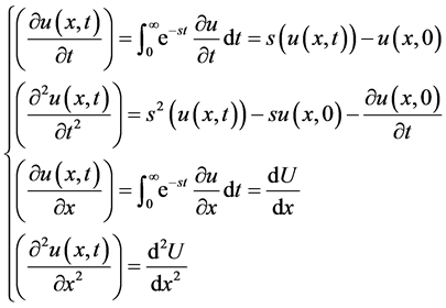
2.1. The Laplace Transform [2]

Let’s note the laplace transform by

(2)

From (1), we have:

(3)

2.2. Laplace-Adomian Decomposition Method (LADM) [3] - [6]

Suppose that we need to solve the following equation:

(4)

subject to initial conditions:

(5)

E is a Banach space, where is a linear or a nonlinear operator, and u is the unknown function.

Let’s suppose that operator F can be decomposed under the following form:

(6)

where is linear, N nonlinear. Let’s suppose that L is inversible to the sense of Adomian with as inverse.

From above, by applying the Laplace transform to both sides of Equation (4), we have:

(7)

From the Equation (7), it follows:

(8)

and this equation gives

(9)

So, from the above Equation (9), we can write:

(10)

We have now:

(11)

We research solution of (4) in the following series expansion form

(12)

and we consider

(13)

where are the Adomian polynomials of and it can be calculated by formula given below.

(14)

Using Equation (12) and Equation (13) in Equation (11) we have:

(15)

From (15), we have the following Adomian algorithm:

(16)

and we obtain the Adomian algorithm:

(17)

Remark

In order overcome the short coming, we assume that can be divided into the sum of two parts namely and. Therefore,we get:

(18)

Instead of the iteration procedure Equation (17) we suggest the following modifi- cation

(19)

The solution through the modified Laplace decomposition method highly depends upon the choice of and.

2.3. He-Laplace Method [7]

We consider a general nonlinear non homogeneous partial differential equation with initial conditions of the form

(20)

N represents the general nonlinear differential operateur and is the source term.

Taking the Laplace transform on both sides of (20), we obtain:

(21)

Û

(22)

Applying the initial conditions given in (22), we have:

(23)

Operating the inverse Laplace transform on both sides of (23), we have

(24)

Now, we apply the homotopy perturbation method

(25)

and the non linear term can be decomposed as

(26)

for some He’s polynomials that are given by

(27)

Sustituding Equation (25) and Equation (26) in Equation (24), we get

(28)

Comparing the coefficients of like powers of p, we have the following approxima- tions:

(29)

3. Illustrative Examples

To demonstrate the applicability of the above-presented method, we have applied it to two linear and two non linear partial differential equations. These examples have been chosen because they have been widely discussed in literature.

3.1. Example 1

Consider the following linear Klein-Gordon equation

(30)

3.1.1. Application of the LADM

Applying the Laplace transform on both side of Equation (30) with the initial con- ditions, we have:

(31)

The inverse Laplace transform give us:

(32)

Û

(33)

We suppose that solution of (30) has the following form:

(34)

From (34) and (33). we have:

(35)

This result garantee that the following Adomian algorithm is:

(36)

Consequently,we obtain:

(37)

So that the solution of (30) is given by

(38)

which is the exact solution of problem.

3.1.2. Application of the He-Laplace Method

Applying the Laplace transform on both side of Equation (30) with the initial con- ditions, we obtain:

(39)

By applying inverse Laplace transform, we have:

(40)

(41)

Now applying the homotopy perturbation method, we have:

(42)

Comparing the coefficient of like powers of p, we have

(43)

which gives us

(44)

So that, the solution is given by:

(45)

3.2. Exemple 2

Consider the following nonlinear Klein-Gordon equation

(46)

where.

3.2.1. Laplace-Adomian Method

Using the Laplace transform, we have

(47)

Û

(48)

by applying inverse Laplace transformation to Equation (48), we hace

(49)

Supposing that the solution of (46) has the following form:

(50)

and

(51)

Taking (50) and (51) in to (49), we obtain:

(52)

According to the standard Adomian algorithm (52), we need to chose

. Here, we choose by convenience So, we

have the following Adomian algorithm

(53)

then garantee that:

(54)

So the exact solution of (46) is

(55)

3.2.2. He-Laplace Method

Using the Laplace transform, we have:

(56)

Now, we apply the inverse Laplace transformation to Equation (46), we have:

(57)

Applying the homotopy perturbation method, we have:

(58)

where are He’s polynomials. The first few components of He’s polynomials are given by

(59)

Comparing the coefficients of the like powers of p, we have:

(60)

(61)

(62)

So that, the exact solution is given by:

(63)

4. Applications

4.1. Problem 1

Consider the following linear Klein-Gordon equation

(64)

Application of the LADM

Using the Laplace transform, we have

(65)

Û

(66)

By appling the inverse Laplace transform, we have:

(67)

Û

Û

(68)

From above equation, we have the following modified Adomian allgorithm:

(69)

Equation (69) give us:

(70)

Thus

(71)

and the exact solution of Equation (64) is

(72)

4.2. Problem 2

Consider the following nonlinear Klein-Gordon equation

(73)

Application of the LADM

Using the Laplace transform from (73), we have:

(74)

Now, we apply the inverse Laplace transform, we have:

(75)

Thus

(76)

Denoting that the solution of (73) has the following form:

(77)

(78)

Taking (77) and (78) into (76), we have:

(79)

and we obtain the following Adomian algorithm:

(80)

Calculation

(81)

Thus

(82)

So that, the solution is given by:

(83)

which is the exact solution of the problem.

4.3. Problem 3

Consider the following nonlinear Klein-Gordon equation

(84)

Application of the LADM

Using the Laplace transform, we have:

(85)

The inverse Laplace transformation is applied to Equation (85) we get

(86)

As before, we defines the solution by the series

(87)

and can be defined by an infinite series

(88)

The nonlinear term is decomposed in term of Adomian polynomials

(89)

Substituting (87), (88) and (89) into both sides of Equation (86) we obtain

(90)

The recursive relation is defined by

(91)

(91) give us

(92)

Thus

(93)

and the exact solution of Equation (84) is

(94)

5. Conclusion

Through these examplles, we showed again the usefulness of Laplace-Adomian Decomposition method and the He-Laplace method, in the search of an approximate solution of Klein-Gordon equation holds for the accepted forms of strong interaction of antiparticles in modern physics.

Cite this paper

Yindoula, J.B., Massamba, A. and Bissanga, G. (2016) Solving of Klein-Gordon by Two Methods of Numerical Analysis. Journal of Applied Ma- thematics and Physics, 4, 1916-1929. http://dx.doi.org/10.4236/jamp.2016.410194

References

- 1. Behe, H.A. (2002) Modern Quantum Theory. 4th Edition, Freeman and Co., San Francisco.
- 2. Fadaei, J. (2011) Application of Laplace-Adomian Decomposition Method on Linear and Nonlinear System of PDEs. Applied Mathematical Sciences, 5, 1307-1315.
- 3. Abbaoui, K. (1995) Les fondements de la méthode décompositionnelle d'Adomian et application à la résolution de problèmes issus de la biologie et de la médécine. Thèse de doctorat de l’Université Paris VI.
- 4. Abbaoui, K. and Cherruault, Y. (1994) Convergence of Adomian Method Applied to Differential Equations. Mathematical and Computer Modellings, 28, 103-109.
- 5. Abbaoui, K. and Cherruault, Y. (1994) Convergence of Adomian’s Method Applied to Non Linear Equations. Mathematical and Computer Modelling, 20, 60-73.
- 6. Abbaoui, K. and Cherruault, Y. (1999) The Decomposition Method Applied to the Cauchy Problem. Kybernetes, 28, 68-74.
http://dx.doi.org/10.1108/03684929910253261 - 7. He, J.H. (2005) Application of Homotopy Perturbation Method to Nonlinear Wave Equation. Chaos, Solitons, Fractals, 26, 295-300. http://dx.doi.org/10.1016/j.chaos.2005.03.006