ABSTRACT

This paper aims at describing the theoretical fundamentals of a reciprocity-based ultrasonic measurement model. This complete inspection simulation can be decomposed in two modeling steps, one dedicated to transducer radiation and one to flaw scattering and echo synthesis. The physical meaning of the input/output signals used in these two modeling tools is defined and the theoretical principles of both field calculation and echo computation models are then detailed. The influence on the modeling results of some changes in the simulated configuration (as the incident angle) or some input signal parameters (like the frequency) are studied: it is thus theoretically established that the simulated results can be compared between each other in terms of amplitude for numerous applications when changing some inspection parameters in the simulation but that a calibration for echo calculation is generally required.

1. Introduction

Ultrasonic techniques are widely used in non-destructive evaluation (NDE) in the aim of characterizing defects in terms of their location, size, type, orientation, etc. It is of great interest to ensure the ability of the methods used to detect and characterize dangerous flaws. Modeling appears to be an efficient technique to improve methods of inspection and data analysis. The modeling of a complete ultrasonic flaw measurement requires the understanding of several different physical processes as well as the connection between them. These processes are notably the description of realistic transducers (the electromechanical transduction), the radiation of waves by these probes, their propagation through complex components, their scattering by arbitrary flaws, the propagation and reception of the scattered waves.

The reciprocity-based relation, whose use in nondestructive testing began with the papers by Kino [1] and Auld [2], provided a general way to make the connection between the different processes involved in an ultrasonic measurement. The measurement modeling approach of Thompson and Gray [3], which is based on Auld’s general relation, allowed the approximate prediction of ultrasonic scattering measurements made through liquidsolid interfaces for relatively small flaws. Schmerr [4] proposed then more complete measurement models which can be used for large flaws.

In parallel, for several years, with the aim of modeling non-destructive evaluation, CEA-LIST and partners have been developing ultrasonic simulation tools which are gathered in the expertise software platform named CIVA [5]. Such tools have been continuously extended through the development of simulation models, from the early nineties, to account for realistic testing configurations in terms of probes (monolithic, phased arrays…), flaws and arbitrary component shapes (canonical shapes, parametrically defined or 2D/3D Computer Aided Design i.e. CAD defined). The existing ultrasonic modules allow to simulate fully real ultrasonic inspection scenarios in a range of applications, which requires the computation of the propagated beam, as well as its interaction with flaws. The beam propagation model is based upon a semi-analytical method which calculates the impulse response of the probe inside the component, assuming individual source points distributed over the radiating surface of the probe. Each elementary source point contribution of the probe toward the computation point is therefore evaluated using a so-called pencil method applied to elastodynamics [6]. This model allows to compute the ultrasonic field in the component for wedge coupled or immersed probes of arbitrary shapes, for monolithic or phased-array transducers. Firstly, developed for homogeneous and isotropic materials, it has been extended to deal with anisotropic and heterogeneous cases [7]. In order to model the scattering of ultrasound by flaws, the choice has been made to adopt mainly analytical approximate or exact methods so as to fulfill requirements of an intensive use. Most of the applied analytical theories (Kirchhoff [8] and Born approximations [9], Geometrical Theory of Diffraction (GTD) [10], Physical Theory of Diffraction (PTD) [11] Separation of Variables (SOV) [12,13]) were already described in a previous reference [14]. The connection between the radiation and scattering modelings is done assuming several hypotheses and using reciprocity considerations, and provides the prediction of flaw responses. The developed flaw response model presents similarities with that described by Schmerr in [4] but also some important differences. The connection between the field and the scattering modeling is carried out here by using a simple field reciprocity principle (detailed in Appendix): the sensitivity of the receiver to a spherical wave scattered from a flaw point M is proportional to the field radiated by the receiver towards the point M. By contrast, Schmerr’s formulation is directly derived from Auld’s reciprocity relation-ship [2] which uses two states, the first one being the current flaw inspection configuration and the second being the same configuration but where the flaw is absent and the previous receiver is now the emitter: as these two states differ by the presence of the flaw, the flaw scattering modeling is directly included in Schmerr’s reciprocity relation contrary to the field reciprocity principle used in this paper. In addition, the choice of the simulation input signal proposed here is very practical: it is simply the experimental specular echo from a reference block (front surface) or from a common large plane calibration reflector (as a Flat Bottom Hole-FBH) located in far field (or in the focal area in case of a focused probe). Contrary to Schmerr’s procedure [4], there is no need to perform a spectral deconvolution to obtain the input signal (called by him “system function”).

In this paper (Section 3), the abilities of the proposed models (for both beam propagation and complete flaws response) are clearly established since it is of great interest notably for NDE industrial applications: the aim of simulation is to help NDE engineers to conceive or optimize the inspection of a specimen including potential flaws by determining the more adequate inspection parameters (incidence angle, wave mode, probe characteristics, frequency…). 

This paper is devoted to the main features description of the proposed measurement model. Sections 2 briefly summarizes the theoretical principles and assumptions used to obtain the formulations for both radiation and flaw response models and the input/output signals of these two modeling tools are clearly defined. The influence of some configurations parameters on the amplitude of simulated results is then studied in Section 3.

2. Physical Definition of Modeling Inputs/Outputs and Basic Principles of the Propagation and Interaction Models

2.1. Field Computation

2.1.1. Description of the Modeling Process

The input signal, as input of the field computation module, corresponds to the time variation of the acoustic particle velocity of the piezoelectric ceramic. The acoustic particle velocity is the component of the vibration velocity normal to the crystal surface.

The output of the field calculation is the displacement at each computation point. Other quantities as the scalar potential for P waves in an elastic solid can be deduced from this displacement.

When computing a field, the model used (pencil method) expresses the absolute amplitude of the simulated field in terms of this particle velocity. Consequently, the model simulates all the propagation phenomena from the outer transducer surface to the field calculation point. The physical phenomena occurring from the coaxial cable to the outer transducer surface (the electro-acoustic transduction) are not taken into account. Moreover, this model is based on a piston-like vibration approximation for the transducer: the particle velocity is supposed to be uniform on the piezoelectric surface. This is an assumption frequently used for transducers modelling. The model process can be represented by a field transfer function (field impulse response) defined as follows:

, (1)

where represents the simulated field (by the way of a scalar quantity) at a computation point M and t is the time of propagation.

2.1.2. Simplified Expression of Radiated Fields

A model has been developed at CEA to predict the ultrasonic field radiated by a transducer (either contact or immersion, monolithic or phased-array) for homogeneous or heterogeneous components made of isotropic or anisotropic materials. This theoretical model is based on a pencil method which has been described in great details in [2] and whose principles, based on Fermat’s principle and energy conservation, are similar to those used in standard geometrical ray theory [15]. In this paper, we will only derive the expressions of the field impulse response in two simple configurations by using another method based on the Rayleigh-Sommerfeld integral for the probe radiation modeling and applying the stationary phase method: these configurations are respectively a fluid medium and an elastic isotropic medium after refraction at a fluid/solid interface. In such configurations, it has been shown in [16] that the pencil method and the Rayleigh-Sommerfeld integral method are equivalent. The pencil method has been chosen for the beam computation module since it can be easily extended to complex components. Nevertheless, the Rayleigh-Sommerfeld integral method presents the advantage to show easily the physics of transducer radiation phenomena in the simple cases.

a)    Field in a fluid medium

For simplification issues, we are interested here in the field radiated by a transducer in a single propagation isotropic medium.

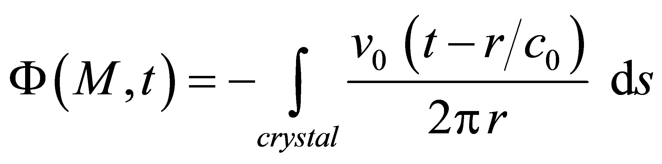
Scalar diffraction theory allows to express the acoustic field in a single fluid propagation medium by the Rayleigh-Sommerfeld integral [17]:

, (2)

where is the velocity potential at point M and at a time t and where and are respectively the distance between a source point S on the surface transducer and the observation point M and the wave speed in the propagation medium. The Rayleigh-Sommerfeld integral expresses physically the beam radiated by a transducer as the superposition of hemispherical waves generated by source points located on the transducer surface.

The previous formula differs from those given by Stepanishen (see Equation (7) in [17]) by the sign minus since we adopt in this document a different definition for the scalar velocity potential for P waves than this author: contrary to Stepanishen (see Equation (2) in [17]), we adopt a more usual definition:

. (3)

It is possible to define the emitter field impulse response as the velocity potential produced at point M by the transducer subjected to a particle speed. The radiated field can be modelled by an impulse response filter, since the emitted potential has the form:

, (4)

where

. (5)

b)    Field in an isotropic medium after a refraction at the coupling/specimen interface

A homogeneous specimen composed of an isotropic medium is then considered.

The previous Expression (4 ) of the Rayleigh-Sommerfeld integral established in the acoustic case can be extended to the refracted field radiated by a probe inside a specimen made of an isotropic material. This extension can be demonstrated as follows (see [16] for more mathematical details). First, in the Rayleigh-Sommerfeld integral, Weyl’s decomposition of a spherical wave in terms of an angular spectrum integral representing a superposition of plane waves is applied. The previous integral has the form of a spatial Fourier transform. Using the stationary phase method, this integral is evaluated by calculating only the contribution of the stationary phase point which corresponds to a particular direction of the wave vector, that of the transmitted geometrical path, respecting Fermat’s principle. The longitudinal elastic field can be expressed as follows: 

(6)

where

, (7)

where we note 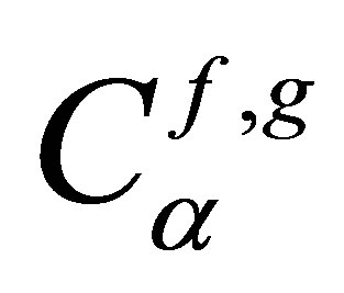with 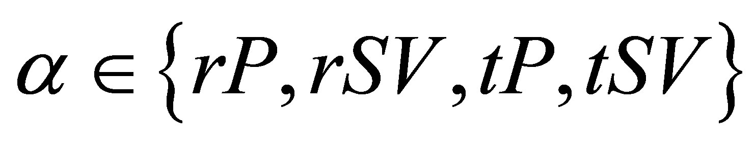the coefficient for reflection (r index) or refraction (t index) for plane waves in harmonic regime related to scalar quantities (f) and (g) (describing the f incident wave and the g refracted wave). For simplification, only this coefficient value at the most representative incident angle will be considered. And, for a mode, is the emission divergence factor and is the time of flight between the source point and M.

.(8)

where is the refracted angle and and are respectively traveled distances along the rays paths in liquid and solid media as defined in Figure 1 . The speeds and density in the specimen material are respectively denoted and. and are the sound velocity and density in the coupling material (assumed here to be a fluid).

Since the transmission coefficient is real for P waves below the critical angle, the incident wave form will not be distorted at the coupling/specimen interface.

In the case of shear waves, for an incident angle between the longitudinal and transverse critical angles, the harmonic transverse transmission coefficient is complex. The scalar potential corresponding to SV waves produced at point M is:

, (9)

with

. (10)

By expressing, for a positive frequency, the transmission coefficient as

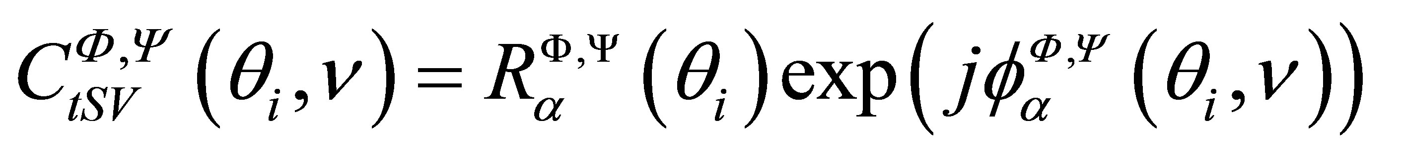it can be shown that, unlike the case of a longitudinal wave, the waveform relative to the SV refracted field (in the focal region of a focused transducer or in the far field of a plane one) is in good approximation not directly proportional to the particle velocity but is the result of a time convolution of this speed with a time function depending on the transmission coefficient phase at the coupling/specimen interface. This function will correspond to the phase distortion of a plane wave refracted into a shear wave at the interface for an incidence beyond the longitudinal critical angle where the refracted P wave becomes evanescent.

Indeed the waveform relative to the SV refracted field is:

(11)

2.2. Defect Response Modeling

2.2.1. Description of the Modeling Process

Unlike the calculation field, the echoes simulation of a given flaw inspection configuration doesn’t directly admit a physical data as input since its entry is a signal obtained from an experimental echo due to the specular reflection on a calibration flaw. Indeed, this reference echo seems to have no direct relation-ship with the current flaw inspection to simulate since the calibration can use a different flaw than the current one and be carried out in a different inspection configuration. Nevertheless, the input signal for defect response simulation must be chosen to have a link with a physical data. Indeed, as shown in Section 2.2.3, this input signal is chosen so as to be equal to the second time derivative of the acoustic particle velocity characterizing the vibration of the single or two identical transducers used in the current inspection:

. (12)

The echoes calculation needs consequently to perform an experimental measurement on a calibration reflector to obtain the input signal for the simulation. Usually, a flat bottom hole or a side drilled hole is employed in that aim.  

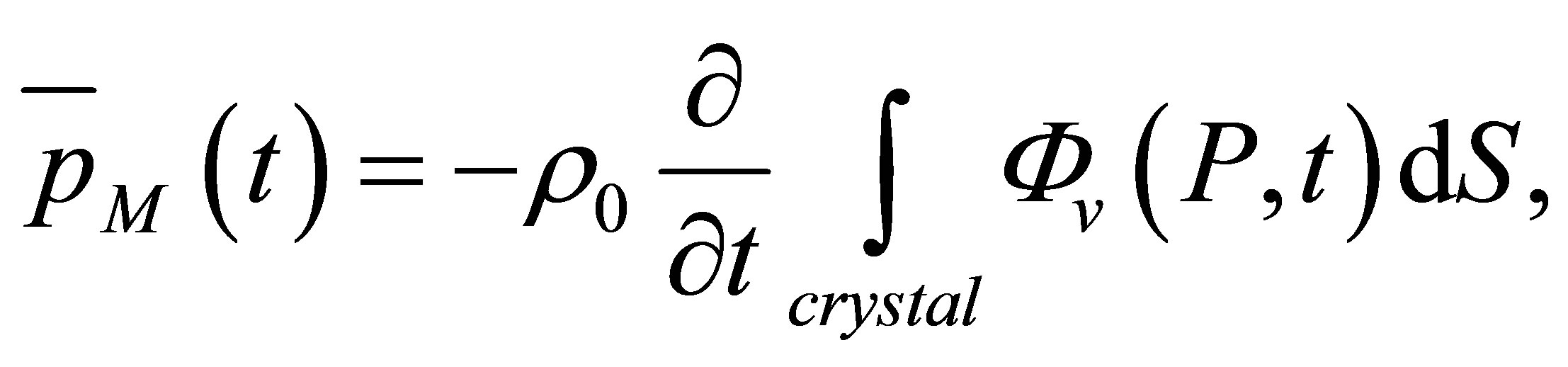
The output of the Defect response module is the total strength applied on the receiving transducer surface:

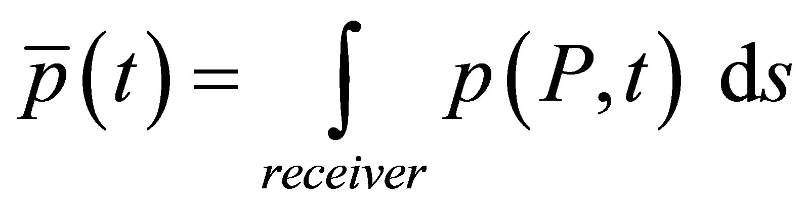. (13)

Here P is one mesh point of the receiver surface, is an elementary surface on the receiver surrounding the point P and is the acoustic pressure at P.

We assume that the measured echographic response is proportional to the total force acting over the receiver surface. The model used for echo computation theoreticcally expresses an echo generated by a flaw in terms of the second time derivative of the acoustic particle velocity (i.e. the input signal for echo computation). From now, we will indeed suppose that the incident field observation point M will belong to the flaw and so M will denote the flaw. So the total strength on the receiver in time domain is modeled thanks to a transfer function (the echographic impulse response from a defect noted M for simplification issues):

. (14)

Consequently, the model simulates all the propagation phenomena from the outer emitter surface to the receiver surface. The electro-acoustic transduction is not taken into account for both emitter and receiver.

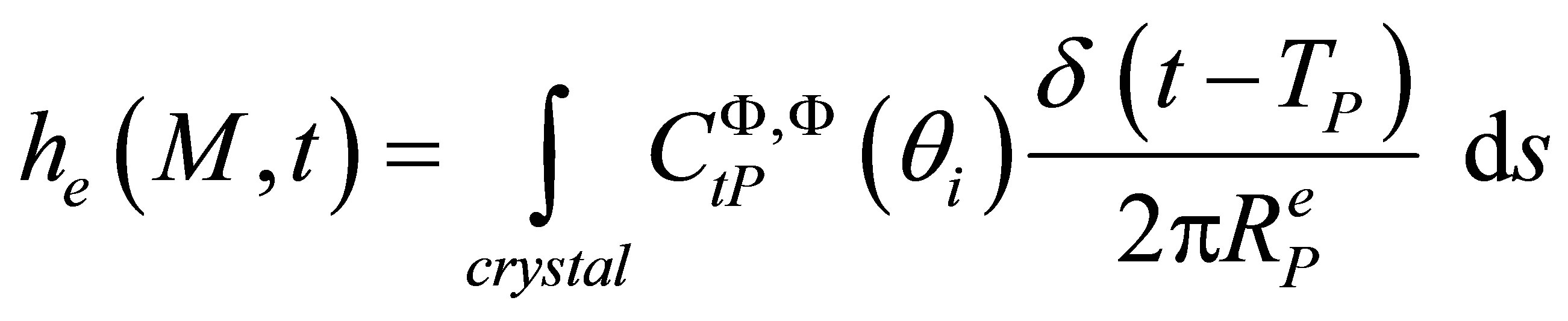
The theoretical expression of the echographic impulse response from a defect is established in next section and in Appendix in the case of a direct P wave echo and given by Equation (A.24).

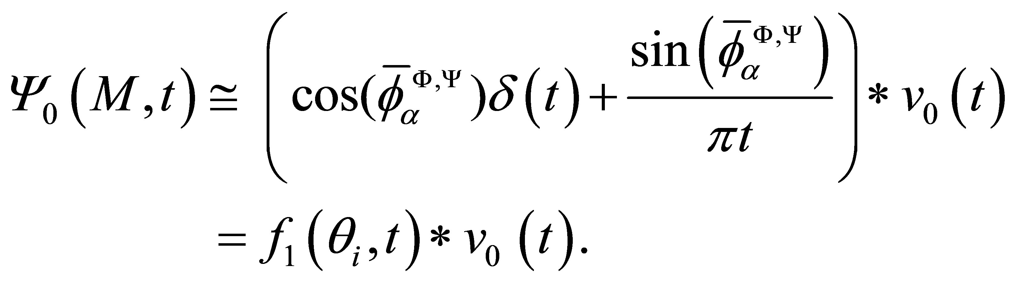
a)    2.2.2. Expression of the Direct Echo Backscattered by a Flaw@NolistTemp# b)    P backscattered echo

Then the defect response model calculates the echoes scattered by a flaw. We report here the main general assumptions applied to deal with the application under consideration. The beam computation model computes the transient bulk wave incident beam using the pencil method. But a simplified description of the so modeled field is assumed for the echo modeling process and only some information (listed later) extracted from the beam computation are used for echo calculation. Indeed the ultrasonic field radiated by the transducer and computed by the beam computation model is approximated by the product of a spatial function describing the amplitude module distribution in the beam and a timedependent function describing the wave propagation. For P waves, this time function is approximated by the particle velocity, both time and phase shifted. This pulse phase distortion is well taken into account in the defect response model but is not mathematically represented in the following formalism for stereographical simplification. Although there’s no signal phase distortion for P waves due to the refraction at the coupling/ specimen interface (contrary to SV waves beyond critical incidence), a phase shift, compared to the velocity particle of the P wave field signal, can be observed for instance for a field computation point far from the probe focal axis; it is due to the summation of time shifted contributions from all the probe sources appearing in the Rayleigh-Sommerfeld field representation. The previous field simplification assumes in fact that the wave fronts in the beam are locally plane in the vicinity of a point M of a flaw: it is usually valid in far field of the emitter or in its focal area if focused. The incident field on this flaw point (in terms of velocity potential) can therefore be approximated as:  

(15)

in which are the co-ordinates of the point M in a frame. The quantities extracted from the field calculation are the function, the time of flight, the signal phase shift and the mean polarization and wave vector directions. The previous directions are used as inputs of the scattering models.

The scattering models we applied are described in great details in [14]. Let just say here that the flaw centred in M is assumed to scatter, at a point M’ in the specimen, a spherical P wave which is characterized by a certain directivity pattern and a spherical SV wave characterized similarly by.

The P and SV scattered fields (in terms of velocity potential) are:

, (16)

. (17)

and depend on time, on the flaw shape and size and incident and observations directions.  

Such an approximation for the scattered field by a flaw is accurate if the defect is located in far field of the receiving probe. Indeed, at an observation point located at a distance of many wavelengths from the flaw, the flaw acts like a point source generating a spherical wave.

It can be shown in Appendix that the P-P pulse-echo amplitude is:

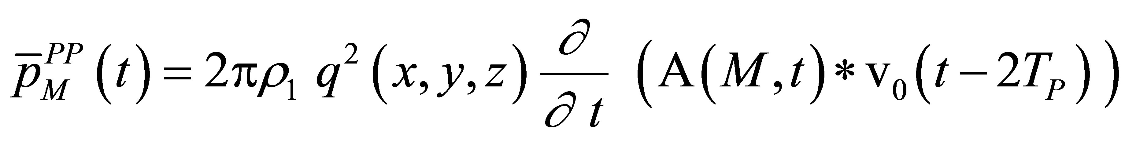. (18)

Such an expression can be obviously extended to pitch-catch configurations. In case of a P- > P wave, the waveform echo derives therefore directly on the particle speed which is convolved with the scattering operator and then time derived. The echo expression is easily rewritten versus the reference signal using (12) :

(19)

If there’s no phase distortion at the coupling/specimen interface (usually the case for P wave field near the focal axis), a phase shift (if observed) in the direct echo signal is only due to the scattering by the flaw.

c)     SV backscattered echo

We define as the SV-SV scattering operator. It can be shown in a similar manner than for P waves that the SV-SV pulse-echo amplitude is:

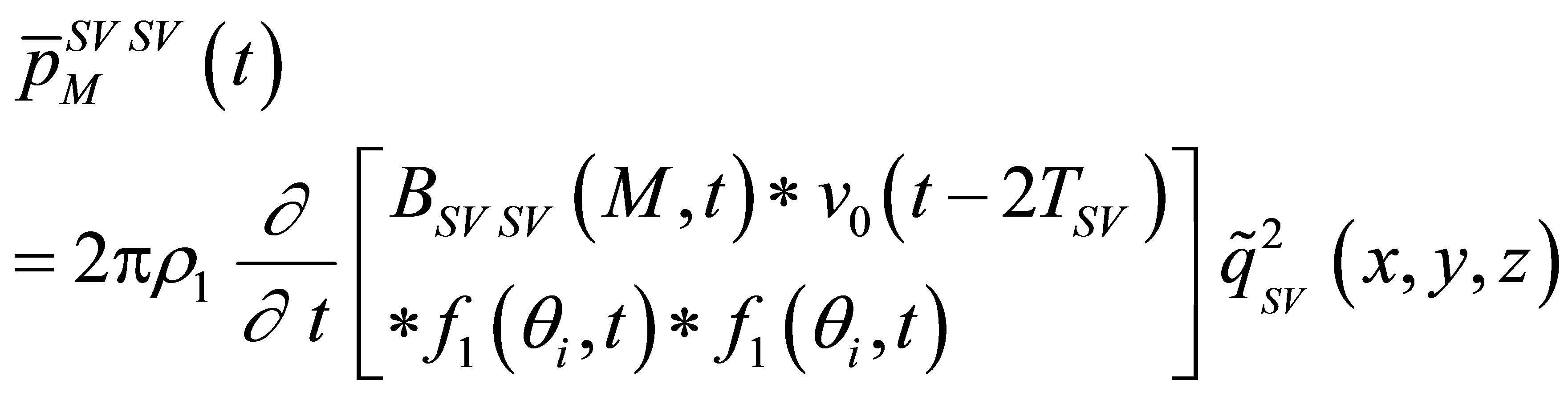(20)

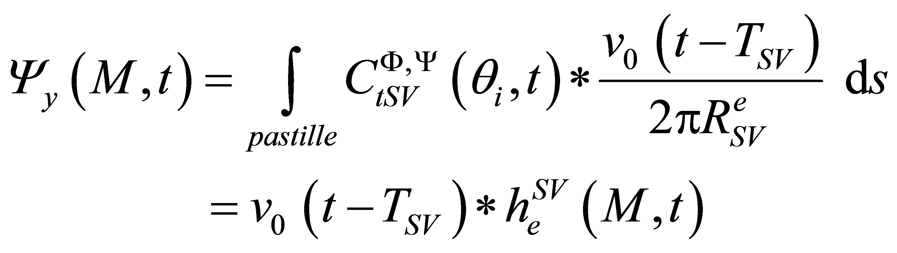
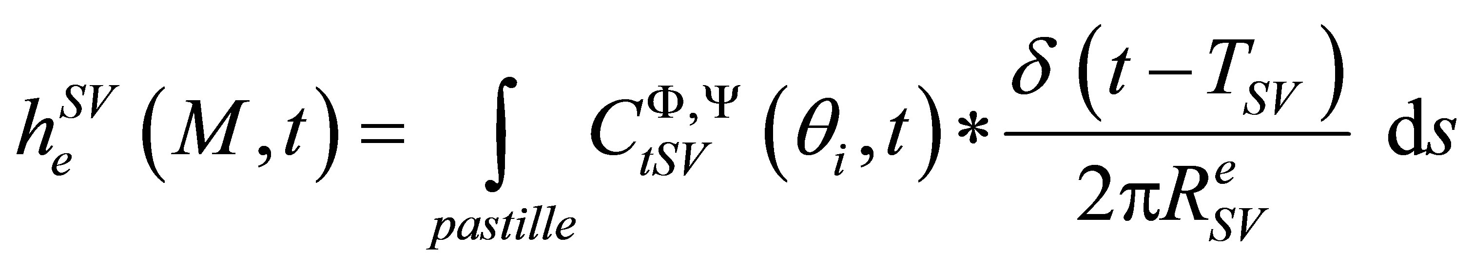
is the spatial function describing the amplitude module distribution in the refracted SV beam. The echo expression is easily rewritten with respect to the reference signal:

(21)

With respect to the input signal, a phase distortion can be observed in the simulated echo due to:

• the P->SV refraction at the coupling/specimen interface. The phase shift at the coupling/specimen interface (related to) takes place twice, one for emission and one for reception.

• the scattering from the flaw.

2.2.3. Calibration

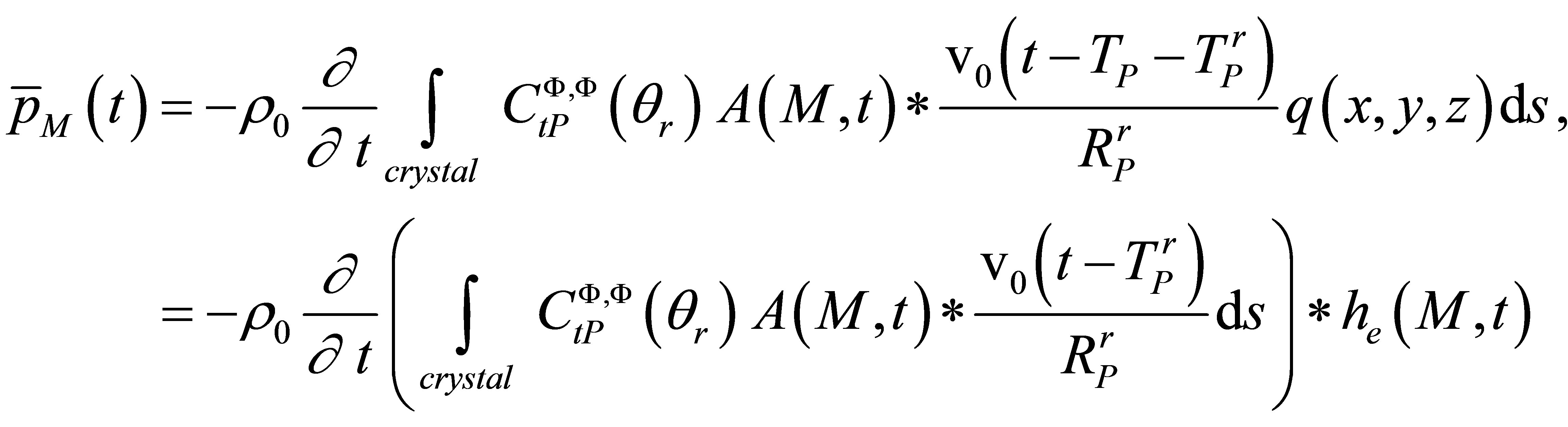
When using an amplitude calibration, the output echo amplitude of the current modeled flaw is normalized by the reference flaw amplitude and this amplitudes ratio corresponds to the ratio of the received electrical signals for the current and calibration defects. The reference specular echo from a large plane surface (entry specimen surface or FBH) can be accurately modeled by the Kirchhoff approximation [8], a high frequency model valid for large flaws compared to the wavelength. Using Equation (10.45) in [4], the reference scattering operator in terms of velocity potential is then given as follows in the case of P waves, S being the calibration target surface:

(22)

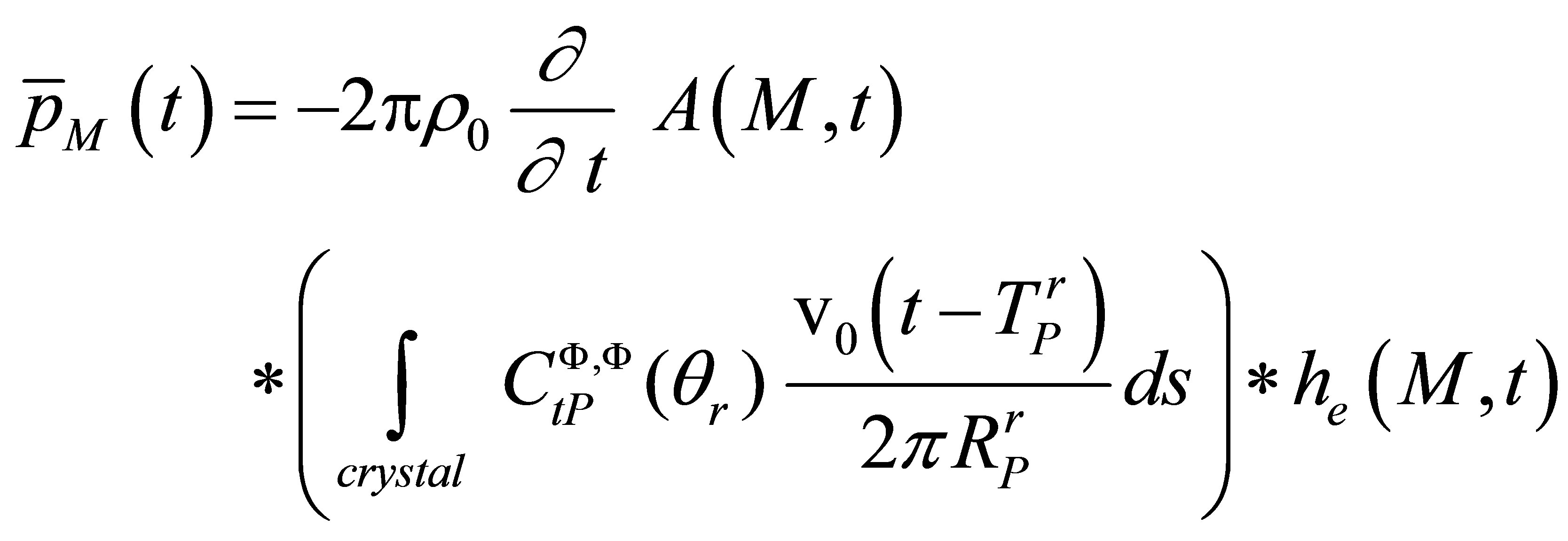
From Equation (A.22), it comes:

(23)

Consequently, the calibration echo from the reference large plane target is directly proportional to the second time derivative of the acoustic particle velocity and the choice stated by (12) for the input signal is justified:

(24)

Contrary to Schmerr’s one, the chosen input signal is simply the experimental specular echo from a reference block (front surface) or from a common large plane calibration reflector (FBH) located in far field (or in the focal area in case of a focused probe). Contrary to Schmerr’s procedure (see Equation (7.4) in [4]), a spectral signal deconvolution of the reference echo by a modeled echographic impulse response is not required thanks to the simple use of the Kirchhoff approximation. Indeed, the choice of the input signal (Equation (12) ) is sufficient to characterize the probe electro-acoustic transduction since it is directly linked to the probe output velocity.

3. Influence of Some Configurations Parameters on the Amplitude of Simulated Results

We will determine here if we can compare the amplitudes between several simulations, when changing some inspection parameters. The influence of several simulation parameters on simulated results will be studied.

For the case of the beam computation module, the objective of field computations is rather to estimate beam sizes or to evaluate beam variations when changing several inspection parameters. The precise knowledge of the input signal (particle velocity) is not required. The use as input signal of a signal deduced from manufacturers’ data (centre frequency, bandwidth) will be sufficient. In this section, for the beam computation module, it is the absolute amplitude of the simulated results which will be compared between several simulations.  

For the case of the defect response model, the amplitude comparison will be operated on the relative (normalized) amplitude of the simulated results which will be compared here between several simulations. The normalized amplitude of an echo signal is the ratio of the absolute amplitude of this signal by the amplitude of a simulated echo from a calibration target.

3.1. Comparison between Two Different Inspection Configurations at the Same Frequency Using the Same Transducer

This case means that we want to compare the simulated amplitudes for two different configurations using the same transducer, for instance by changing the incident angle of the probe or by replacing the coupling or specimen material.

Since the same probe is used, the different simulations will be carried out by choosing the same input signal for each calculation. The term transducer refers to the piezoelectric element and consequently using the same transducer induces no change in the piezoelectric material and in its shape (all the dimensions of the crystal). It is recalled that the crystal thickness is directly linked to its resonance frequency and so to the centre frequency of the probe.

3.1.1. Field Computation

In such a comparison, there’s no change in the acoustic particle velocity since the same transducer is used in the different configurations. Consequently, the absolute amplitudes of the simulated fields radiated in the different configurations can be compared.

3.1.2. Defect Response Model

The electro-acoustic transduction is identical for these two configurations with the same transducer. So it is possible to compare the normalized amplitudes of different simulations in order to evaluate the sensitivity of echoes amplitude to one or several parameters. The reference measurement (used to fix the input signal and the normalization amplitude) can be carried out for instance in one of the simulated configurations we would want to compare.

In conclusion, for the two ultrasonic models, we can evaluate in simulation with a good precision the influence of simulation parameters (as replacing the incident angle or the specimen material).

3.2. Comparison between Two Different Inspection Configurations at the Same Frequency Using Two Transducers of Same Thickness but Different Aperture Dimensions

The conclusions are similar to the previous case (same dimensions) since we can suppose in a good approximation that the electro-acoustic transduction and the particle velocity don’t vary with respect to the crystal aperture dimensions (for instance, the diameter for a circular probe). Indeed, the model assumes that the transducer acts as a piston: the velocity is uniform on its surface, whatever the size and the shape of the radiating surface.

3.3. Change in the Signal Centre Frequency

In that case, the input signal differs from one simulation to the other. The electro-acoustic transduction is not modeled in the developed tools: moreover it varies from one transducer to the other and consequently depends on frequency.

3.3.1. Beam Computation

Since there’s no account of electro-acoustic transduction, the frequency effects on the propagation phenomena occurring only between the transducer surface and the beam computation point can be evaluated. Consequently, the variation versus frequency of the radiated beam characteristics (for instance the beam focal width or divergence) can be estimated. 

3.3.2. Defect Response Model

For the defect response model, when comparing several simulations at different frequencies, all the propagation and interaction phenomena between the emitting and receiving cables (notably the electro-acoustic transduction) can be taken into account so as to better approach the physical reality. Indeed, we relax the absence of modeling of the electro-acoustic transduction, by comparing the variation with frequency of the ratio of echoes amplitudes from a defect and a calibration flaw. As the echo amplitude from the calibration flaw will in all cases depend on frequency, this method will not show only the variation with frequency of the echo amplitude from the defect of interest.

The procedure to follow in order to study at different frequencies the ratio of echoes amplitudes from a defect and a calibration flaw is given hereafter. An echo computation is supposed, in the view of reproducing the physical reality, to be completed by a measurement on a calibration flaw. This measure must be carried out at each frequency to choice the valid input signal in the simulation. In order to evaluate the frequency variation observed on echoes calculations (and eventually to compare it with measure), it is needed to:

• make measurements at each frequency: one on the current defect and one on a calibration reflector.

• perform simulations of these two measurements, using in modeling an input signal deduced from the experimental echo on the calibration reflector at each frequency.

• normalize at each frequency the echoes amplitudes by those of the reference defect both on experimental and simulated data.

In conclusion, the variation with frequency of the ratio of echoes amplitudes from a defect and a calibration flaw can be studied thanks to the developed defect response model.

3.4. Comparison between Two Different Transducers Radiating at the Same Frequency

The conclusion is the same as for the effect of a change in the centre frequency.

4. Conclusions

A complete reciprocity-based ultrasonic measurement model has been designed to simulate ultrasonic NonDestructive Evaluation (NDE); it can also be used for other applications of ultrasonic echography as telemetry [18]. The two components of this model (beam computation and defect response model) have been theoretically described. The physical meaning of the inputs/outputs used in these modeling modules has been defined. Then it has been theoretically shown that the simulated results can be compared between each other in terms of amplitude for numerous applications when changing some inspection parameters in the simulation. For instance, the comparison of simulated amplitudes can be performed for both fields and echo models when using the same transducer but changing in simulation the incident angle, or the coupling or specimen material. The previous abilities of the developed model are of great interest for industrial NDE simulation which is commonly used to optimize the parameters of inspection (incidence angle, wave mode, probe characteristics, frequency…) of a specimen including potential flaws.

As to the complete measurement model, it has been pointed out that it is needed to make a calibration measurement on a reference flaw to avoid the electroacoustic transduction modeling. Such a calibration allows to study frequency effects by simulating the frequency dependency of the ratio of echoes amplitudes from the current and the reference flaws. The proposed model offers the possibility of a very simple choice for the input modeling signal: this signal is directly taken as the experimental echo on a large planar reference target. Experimental validations of this simulation tool have been successfully performed [5,19].

5. Acknowledgements

This work was supported by EXTENDE.

REFERENCES

Appendix

Echo modeling and field reciprocity principle

The aim of this appendix is to establish in the case of P waves (longitudinal wave incident on the defect, longitudinal wave diffracted) the expression of the corresponding echo which is linked to the average pressure on the receiving transducer surface.

The scattered velocity potential at a point M’ in the solid specimen has been defined as:

. (16)

Moreover we already expressed the incident field as follows:

(15 )

Thus

(A.1)

The velocity potential diffracted by the defect is at a point P in the liquid medium after the refraction at the solid-liquid interface: 

, (A.2)

where the time of flight and divergence factor for reception are :

(A.3)

For simplifications issues, we will consider in the following that a coefficient (respectively) corresponds to the transmission coefficient at the liquid-solid interface for the emission path (respecttively solid-liquid interface for the reception path). and are the incident and refracted angles at the solid->liquid interface for the reception path. These angles depend on the corresponding path included in the probe aperture. and are the propagation distancesin the solid and fluid media. In the case of a P wave incident on a solid-liquid interface with an incident angle less than the longitudinal critical angle, the transmission coefficient in harmonic regime is always a real which does not depend on frequency. It is also the case for the emission transmission coefficient.

The electrical signal measured at the receiver output is proportional to the average pressure on the transducer. We will now express the simulated echo which is the total force applied on the receiver surface (product of the average pressure by the transducer area):

(A.4)

The previous expression represents the calculation of the total strength applied on the receiver surface versus the velocity potential (scattered by the flaw in M) on each point P of this surface. The previous expression is obtained from the following relation demonstrated just after which connects the pressure and the velocity potential:

(A.5)

Using the Bernoulli's equation on the velocity:

(A.6)

and:

(A.7)

we obtain the relation (A.5 ) to demonstrate since:

(A.8)

From the previous Equations (A.1) and (A.5 ), it comes:

(A.9)

We assume now that is constant over the receiver surface:

(A.10)

The integral of the previous formulation corresponds to the receiving transducer response (i.e. the field in reception). This integral is similar to that expressing the incident field potential radiated at the point M and differs only by a proportionality factor, as shown in Equation (6) . This similarity expresses a field reciprocity between emission and reception.

In the following, we will calculate the proportionality factor and show the simplifications obtained due to reciprocity considerations.

(A.11)

with

(A.12)

is called the reception impulse response and corresponds to the sensitivity of the receiver to a spherecal wave source located at point M. We can also define the receiver field impulse response as the velocity potential produced at point M by the receiving transducer considered as an emitter and subjected to a particle speed:

(A.13)

The field radiated by the receiver at point M is directly in terms of velocity potential.

We will show now that the reception impulse response previously involved in the echo formulation is proportional to the receiver field impulse response. Indeed, differs from only by the transmission coefficient and the divergence factor (inside the integral) which are calculated in a direction from point M to the transducer rather than the opposite. 

For notations simplification, we will consider now a pulse echo configuration to express easier the reciprocity between transmission and reception (it could be demonstrated in a same manner for other kind of configuretions). In pulse echo and for P waves, and thus:

(A.14)

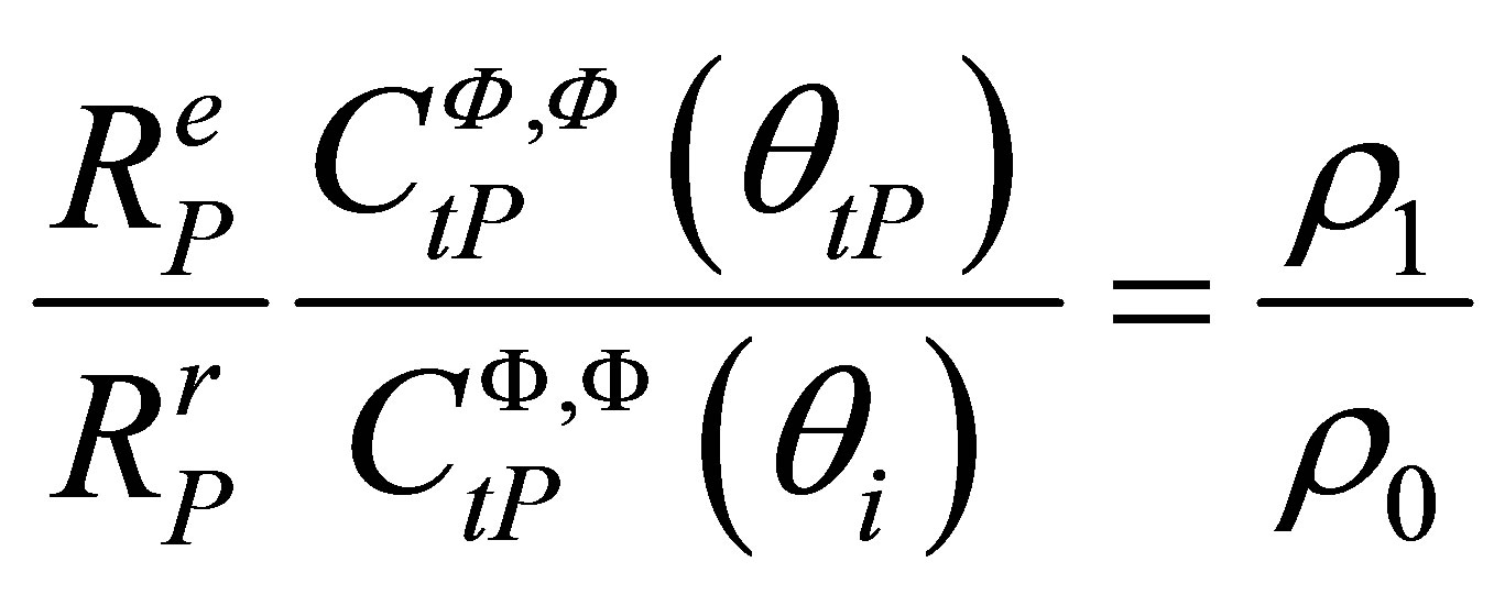
A reciprocity relation can be obtained for transmission coefficients [18] involved in emission and reception:

(A.15)

where is the density of the solid and and are the oblique impedances respectively in the liquid and solid media for longitudinal waves.

A reciprocity relation can also be obtained for divergence factors involved in emission and reception:

(A.16)

We finally obtain:

(A.17)

This ratio is a constant which doesn’t depend on the incident angle and so on the path linking the point M to one source point on the transducer.

This following proportionality between these impulse responses expresses the reciprocity between emission and reception:

(A.18)

In pulse echo configuration, the emitter and receiver are identical and

(A.19)

(A.20)

The expression of the total force applied on the receiver is finally from (A.11) :

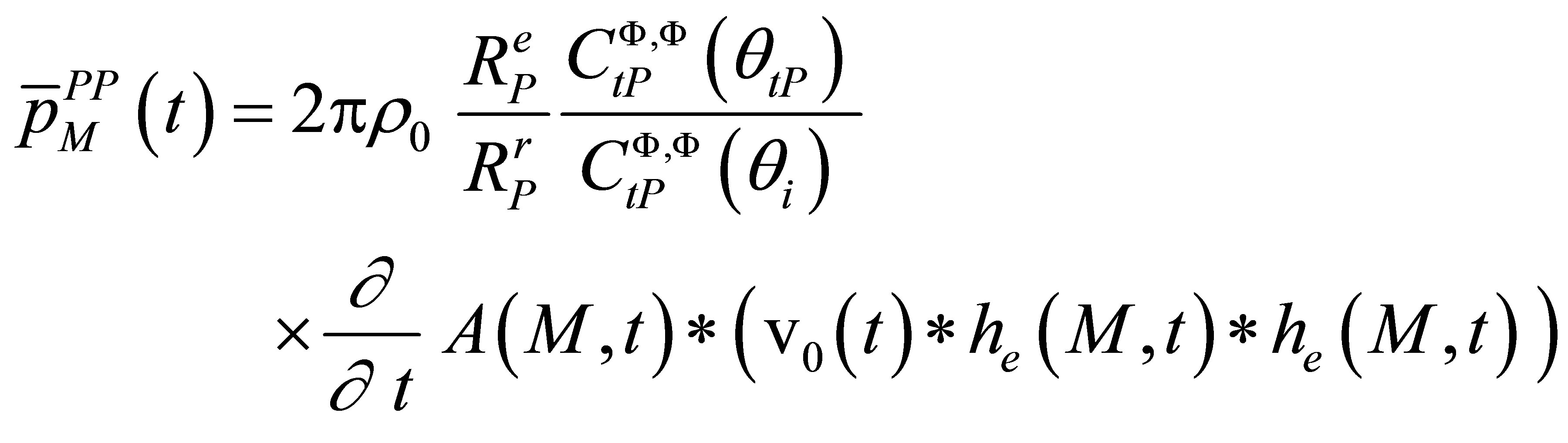(A.21)

and then

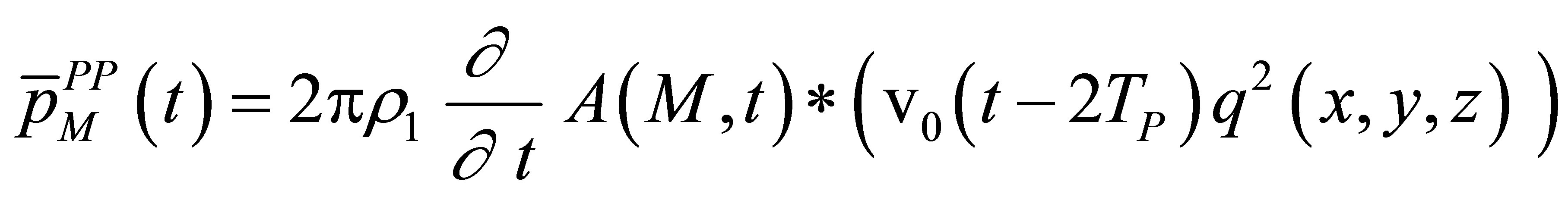(A.22)

The P wave echo is proportional to the square of the spatial distribution of the radiated field potential. The echo waveform is obtained from the particle velocity by convolution with the flaw impulse response (scattering operator) and a time derivation. We can express the echo versus the input reference signal:

(A.23)

The above equation describes the relationship between the output and input of the defect response model for P waves in a pulse echo configuration.

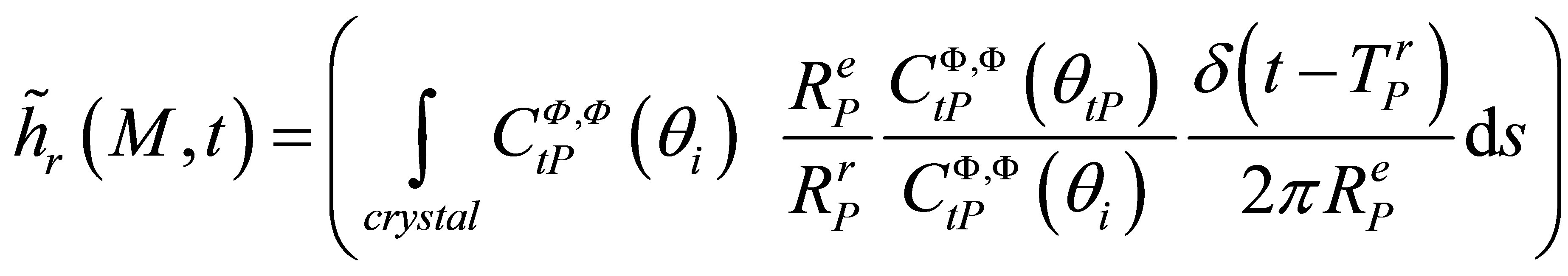
We can finally establish the expression of the echo graphic impulse response from the defect:

(A.24)

REFERENCES

- G. S. Kino, “The Application of Reciprocity Theory to Scattering of Acoustic Waves by Flaws,” Journal of Applied Physics, Vol. 49, No. 6, 1978, pp. 3190-99. doi:10.1063/1.325312
- B. A. Auld, “General Electromechanical Reciprocity Relations Applied to the Calculation of Elastic Wave Scattering Coefficients,” Wave Motion, Vol. 1, No. 1, 1979, pp. 3-10. doi:10.1016/0165-2125(79)90020-9
- R. B. Thompson and T.A. Gray, “A Model Relating Ultrasonic Scattering Measurements to Unbounded Medium Scattering Amplitudes,” Journal of the Acoustical Society of America, Vol. 74, No. 4, 1989, pp. 1279-1290. doi:10.1121/1.390045
- L. W. Schmerr, Jr. and J. S. Song, “Ultrasonic Nondestructive Evaluation Systems: Models and Measurements,” Springer, New York, 2007. doi:10.1007/978-0-387-49063-2
- CIVA Software Website. http://www-civa.cea.fr
- N. Gengembre and A. Lhémery, “Pencil Method in Elastodynamics. Application to Ultrasonic Field Computation,” Ultrasonics, Vol. 38, No. 1-8, 2000, pp. 495-499. doi:10.1016/S0041-624X(99)00068-2
- N. Gengembre and A. Lhémery, “Calculation of Wideband Ultrasonic Fields Radiated by Water-Coupled Transducers into Heterogeneous and Anisotropic Media,” Review of Progress in QNDE, Vol. 19, 2000, pp. 977-984.
- R. Chapman, “Ultrasonic Scattering from Smooth Flat Cracks: An Elastodynamic Kirchhoff Diffraction Theory,” CEGB Report, North Western Region NDT Applications Centre, 1982.
- M. Darmon, P. Calmon and B. Bele, “An Integrated Model to Simulate the Scattering of Ultrasounds by Inclusions in Steels,” Ultrasonics, Vol. 42, No. 1-9, 2004, pp. 237-241. doi:10.1016/j.ultras.2004.01.015
- M. Darmon, S. Chatillon, S. Mahaut, L. Fradkin and A. Gautesen, “Simulation of Disoriented Flaws in a TOFD Technique Configuration Using GTD Approach,” 34th Annual Review of Progress in Quantitative Nondestructive Evaluation, 2008.
- V. Zernov, L. Fradkin and M. Darmon, “A Refinement of the Kirchhoff Approximation to the Scattered Elastic Fields,” Ultrasonics, Vol. 52, No. 17, 2012, pp. 830-835. doi:10.1016/j.ultras.2011.09.008
- C. C. Mow and Y. H. Pao, “The Diffraction of Elastic Waves and Dynamic Stress Concentrations,” Rand Corporation, Santa Monica, 1971.
- C. Ying and R. Truell, “Scattering of a Plane Longitudinal Wave by a Spherical Obstacle in an Isotropically Elastic Solid,” Journal of Applied Physics, Vol. 27, No. 9, 1956, p. 1086. doi:10.1063/1.1722545
- M. Darmon, N. Leymarie, S. Chatillon and S. Mahaut “Modelling of scattering of ultrasounds by flaws for NDT,” In: A. Leger and M. Deschamps Eds., Ultrasonic Wave Propagation in Non Homogeneous Media, Springer Proceedings in Physics, Vol. 128, Springer, Berlin, 2009, p. 61-71.
- V. Cerveny, “Seismic Ray Theory,” Cambridge University Press, Cambridge, 2001. doi:10.1017/CBO9780511529399
- N. Gengembre, “Modélisation du Champ Ultrasonore Rayonné Dans un Solide Anisotrope et Hétérogène par un Traducteur Immergé,” Université Paris, 1999.
- P. R. Stepanishen, “Transient Radiation from Pistons in an Infinite Planar Baffle,” Journal of the Acoustical Society of America, Vol. 49, No. 5B, 1971, pp. 1632-1638.
- B. Lu, M. Darmon, C. Potel, “Stochastic Simulation of the High-Frequency Wave Propagation in a Random Medium,” Journal of Applied Physics, Vol. 112, No. 5, 2012, pp. 054902.
- R. Raillon, et al. “Validation of CIVA Ultrasonic Simulation in Canonical Configurations,” 18th WCNDT, 2012.