Theoretical Economics Letters
Vol.05 No.01(2015), Article ID:53727,11 pages
10.4236/tel.2015.51008
Contribution of Education and Innovation to Productivity among Mexican Regions: A Dynamic Panel Data Analysis
Vicente German-Soto1, Luis Gutiérrez Flores2
1Facultad de Economía, Universidad Autónoma de Coahuila Unidad Camporredondo, Saltillo, Mexico
2Centro de Investigaciones Socio-Económicas (CISE), Universidad Autónoma de Coahuila Unidad Camporredondo, Saltillo, Mexico
Email: vicentegerman@uadec.edu.mx, luis.gutierrez@uadec.edu.mx
Copyright © 2015 by authors and Scientific Research Publishing Inc.
This work is licensed under the Creative Commons Attribution International License (CC BY).
http://creativecommons.org/licenses/by/4.0/


Received 15 January 2015; accepted 30 January 2015; published 2 February 2015
ABSTRACT
A dynamic panel data (DPD) model is estimated to assess the contribution of the average schooling years, the education expenditure and the inventive coefficient―as an approximation for innovation―to the increased productivity of the Mexican states. The potential difficulties of endogeneity and serial correlation are controlled by adopting system General Method of Moments (GMM) procedures. The findings are compatible with the theory. The importance of the lags is confirmed and the positive and significant impacts on productivity tend to vary according to the income level and the geographical location of the regions. Innovation is an important contributor to northern, central and richer states’ productivity, but education expenditure is important for the poorer states and scholarly attainment stands out in the southern states. The analysis emerging from the model concludes that these regional differences should be seen as a potential opportunity for designing customized policies capable of increasing the productivity and not as a weakness.
Keywords:
Productivity, Education, Patents, Dynamic Panel Data, Autoregressive Models

1. Introduction
Throughout the period 1994-2012, the Mexican economy accumulated 3.72 patents per 100,000 inhabitants, as an annual average; the educational attainment reached 7.76 years of scholarly attainments and the education expenditure per student at the university averaged 14.67 Mexican pesos at constant prices. However, the gross productivity, assessed as the per capita gross state product (GSP), grew at annual rate of below 3%, an insufficient rate of growth to achieve the necessary employment demanded by the population. Why, if education and innovation have elevated their performance, has the national productivity been very low?
In this work, we seek to respond to this question by assessing the contribution of these factors to the productivity results. We consider that the performances of innovation and educational attainments have been unequal regarding the productivity of the Mexican regions. States with major innovation and education levels must achieve the best results for productivity, while states with low performance in terms of innovation and education obtain inferior levels of productivity. We also explore this relationship by considering two criteria under which the Mexican states are easily identified. Attending to a geographical pattern, the states with better indicators seem to be located in the central and northern regions, while southern and gulf states show the lowest performance. The income-level criterion will allow us to infer if richer and middle-income states exhibit the best adjustment and whether the performance of the poorer states remains behind.
The empirical evidence is supported by executing a dynamic panel data (DPD) model in which it is assumed that the pay-offs of education and innovation in terms of major productivity may appear with a lag, and additionally the past performance of productivity itself plays a potential role in its current values, in such a way that it is also considered as a potential explanatory variable. The difficulties arising from consider autoregressive terms are overcome with the two-stage system GMM procedure and by evaluating the over-identifying restrictions with the J statistic test.
Explanations of human capital theory, pioneered by Becker [1] and Schultz [2] , suggest that education results in enhanced productivity. Education may often act as a signal of productivity (Chevalier et al. [3] ). Employers believe that better educated individuals will bring more productivity and these factors seem to shape a clear relationship. The new growth theory considers that technological change, manifested in a variety of ways, raises productivity. Some specific methods adopted as a result of technological change are the generation of new ideas and new knowledge, learning by doing and finally innovation that emerges after a long process (Paus [4] ). Much of the recent literature on productivity recognizes both education and innovation factors as key elements in elevating productivity and facilitating technological change. Economies with a high education level also tend to achieve a high level of productivity. In this line, high levels of innovation are related to the best performance in terms of productivity. On the contrary, when these factors have poor performance, the levels of productivity are also low. Therefore, education and innovation can be detonators for―or important barriers―development.
Our findings are compatible with the theory. The importance of the lags is confirmed. The estimates report a positive and significant contribution of education and innovation to productivity that tends to vary between rich and poor economies as well as among the geographical locations of the regions.
The rest of the paper presents a review of the literature (Section 2), the econometric methodology (Section 3), a description and exploratory analysis of the database (Section 4), the main results (Section 5), and finally some concluding remarks (Section 6).
2. The Interconnectivity among Education, Innovation and Productivity: A Review
Innovation has become a key issue when trying to understand the effects of the global economy on cities and regions all over the world. Policymakers and academics often relate problems such as unemployment, economic inequality and lack of growth, especially in less developed countries, to the diminished capability of those countries to generate innovative processes or products. From this view, knowledge-based innovation is the spearhead of a successful path to long and prosperous growth (Power and Malmberg [5] ).
Moreover, the sources of productivity growth are a central topic in economic theory and empirical research. Recent literature has emphasized the role of several elements in the supply-side context, such as innovation, physical capital resources, and technology. On the demand side, the determinants of productivity have been analyzed since the publication of the paper by Kaldor and Mirrless [6] . In this arrangement, labor division allows for workers’ skill set to improve, inducing the incorporation of technological innovation and, in combination with more specialization, structural changes in the economy, leading not only to productivity growth but also to further specialization (Crespi and Pianta [7] ).
Behind the aforementioned ideas lies education or schooling. Although referred to indistinctively in many documents, education and schooling are not the same. According to Pencavel [8] , education takes place outside of schools, for example in families, communities and workplaces. Schooling refers to the time invested in acquiring codified knowledge in particular environments, such as classrooms and books, with the aim to improve the quality of the workforce. There has been substantial research regarding the contribution of higher education to a nation’s economic growth at all levels. For instance, growth accounting techniques relate changes in schooling completion levels to changes in aggregate output. Some work has also been conducted using a more microeconomic approach, in order to measure the association between the educational attainments of workers and the productivity growth. The overall results from these empirical efforts tend to confirm the idea that education positively contributes to growth and productivity.
Altogether, innovation and education are considered to be fundamental elements of the “five drivers of productivity growth” (Mayhew and Neely [9] ). Investment in new machinery may embody technical progress (innovation) that will enhance performance. Investment in knowledge (R&D), when adequately adopted in organizational operations, allows labor and capital to be put to more productive use. Investment in human beings, whether in full-time education or in the workplace, increases human capital and makes it more productive. In this context, we can think on innovation as an ongoing and complex process of learning and applying new ideas and technologies. Of course, the referred process deriving from innovation is accumulative and relies heavily on the ability of the country or region to develop such efforts for special factors like the quality of education, the availability of knowledge infrastructure―universities and research centers―and the efficient functioning of the markets (Vieira et al. [10] ). These innovations must be reflected in the competitiveness of countries and regions. The role of universities and their economic potential, as traditional carriers of advanced research and higher education, are being increasingly discussed. At regional levels, the potential of universities to contribute to innovation has led to them being linked more strongly to regions’ innovation and industrial systems. Power and Malmberg [5] mention that universities can contribute to regional innovation in two ways: firstly, universities increase the production of knowledge since they provide the market with new workers and patent scientific results; secondly, the existence of universities can lead to a transfer and exchange of knowledge between the universities and the region’s industrial sector.
Empirically, a large number of works attempt to highlight the relationship between innovation, education and productivity growth. For instance, Pencavel [8] provides a review of research on the contribution of education to productivity for the USA in a non-technical fashion. The author concludes that rising schooling completion levels and movements in the quality of schooling have contributed to the growth of labor productivity in the USA.
Furthermore, Power and Malmberg [5] explore the debate about competitive and prosperous regions and their relationship with universities and higher education. They present an excellent depiction regarding the role of universities in regional economic development and conclude that policy efforts should result in aligning innovation and science and technology policies with regional development. In another context, AlAzzawi [11] examines the effect of foreign direct investment (FDI) on innovation and productivity. He uses patent citations within FDI to measure the degree of access that one nation gains to the R&D knowledge of another. FDI-in- duced R&D spillovers can be very important for developing countries, since they affect both innovation and productivity.
Vieira et al. [10] emphasize the importance of the input of innovation in the production process as a way to maximize the capacity and efficiency of the labor factor, translated into its productivity. Their empirical findings point to a positive influence of innovation and labor productivity in the European regions. Interestingly, investments in R&D are more profitable in less developed regions. In a more detailed context, Harris et al. [12] investigate whether sourcing knowledge from cooperating on innovation with higher education institutions impacts on the establishment-level total factor productivity, and they also evaluate whether this impact differs across Great Britain’s regions and according to the property structure of the firm―domestic or foreign. They use propensity score matching to obtain a positive and significant impact of innovation cooperation on productivity, although there are differences in the strength of the impact in the different regions and depending on the property structure.
In Mexico, some recent documents mark the start of a research area of interest given the relevance of the technology innovation diffusion to productivity and growth, as well as the increased share of the Mexican economy in the global market. Particularly, the works by German-Soto et al. [13] , Ríos Bolívar and Marroquín Arreola [14] , Cabral and González [15] and Brown and Guzmán [16] all attempt to characterize the recent phases of the development and growth process in the country, featuring the innovation aspect. In a somehow related approach, Crespi and Zuñiga [17] examine the determinants of technological innovation and its impact on firm labor productivity for six Latin American countries including Mexico. They find that firms investing in knowledge are more able to introduce technological advances, and those who innovate have greater labor productivity. In a more disaggregated perspective, Mungaray and Ramírez [18] study the effects of human capital on labor productivity for a sample of low value-added microenterprises. They report evidence of the relationship between human capital and labor productivity and conclude that the long-run existence of the firms in the sample can be explained by the accumulation of management experience. Cabral and Gonzalez [15] estimate negative effects from R&D on productivity of a set of Mexican manufacturing sectors. Brown and Guzmán [16] analyze the determinants of innovation of Mexican manufacturing establishments and highlight that innovation has been influenced by characteristics of the open economy such as exportation activities, foreign investments and also it is related to the size of the firm.Because of productivity is considered to be one of the key elements in explaining regional growth and its differences, it will be interesting to explore some of the main factors that determine it.
3. An Overview of the Autoregressive Models and Dynamic Panel Data
The role of time is essential for several phenomena occurring in Social Sciences and Economics. The relationship of dependency among the variables is less instantaneous than one might think for psychological reasons― people and therefore economies do not change their habits immediately, imperfect information―sometimes the market offers consumers all kinds of products and varying features and prices, making them hesitate to buy now and wait until prices decline, and institutional rigidity―for example, contractual obligations and long-term investments, among others. Therefore, a lag time should be considered, especially if a regression equation is used to determine how some variables are linked.
The explicit consideration of the time factor brings to the distributed-lag models. In such models, the effect of a regressor x on y occurs over time:
 (1)
(1)
In Equation (1) the lag polynomial
 is applied to the explanatory variable
 , so it defines a pattern showing how
 affects
 over time.
Of course, it is not possible to estimate an infinite number of terms of
 coefficients in (1). One practical alternative is the solution given by Koyck [19] , who considers that lag effects are geometrically reduced and each value of
 is inferior to each preceding
 . With returns to the past, the effect of the lag on
 is gradually reduced considering a fixed factor, say
 . So, Equation (1) is defined as:
 (2)
(2)
Subtracting Equation (2) from (1) and rearranging terms, the Koyck transformation is:
 (3)
(3)
where , i.e., a moving average of
 and
and . As we can see, the transformation ends with an autoregressive model because one lag of the dependent variable is included as explanatory. With this simplification, Koyck solves two problems. First, only the estimates for
 ,
,
 and
and
 are required, and second, expression (3) solves the potential problems of multicollinearity because only one period of
 is considered in the model and not its several past values.
The dynamic marginal effects of
 on
on
 in this specification are:

The long-run multiplier is assessed by expression , which predicts an exponentially de-
clining lag distribution under the assumption that many economic relationships seem to be adjusted in this way.
The model can be augmented to include more than one regressor. For the case of two regressors,
 and
and , Equation (3) would be defined as:
 (4)
(4)
As before, the dynamic marginal effects of z on y are:

Commonly, we are more interested in the mean and median of the lags with the aim to obtain an idea of the lag structure. In this model, they are estimated as follows:
 ;
; .
.
Here “ln” indicates natural logarithms. These measures can be used as the speed at which
 responds to
 .
.
Equation (4) resumes the theory of autoregressive models when the regression is for time-series structures. Its adequacy in panel data is immediately apparent:
 (5)
(5)
where the residuals
 follow an MA(1) process and the two usual individual and time-specific effects are included,
 and
and ; moreover, Equation (5) considers up to
 explicative variables and the
 are assumed to be independently distributed across individuals with a zero mean.
Equations (4) and (5) have the problem of consistent estimation because the lagged dependent variable as a regressor on the right-hand side is almost never strictly exogenous, as required by the ordinary least square estimator (OLS). Therefore,
 is correlated with the error term and the OLS estimator is biased and inconsistent (Baltagi [20] ) even in the case that
 are not serially correlated.
For dynamic panel data, several solutions have been proposed. Arellano and Bond [21] suggest using the orthogonality conditions that exist between the lagged values of
 and the disturbances
 as instruments in the regression equation. In the two-step GMM estimator, the authors basically use lagged differences of the dependent variable as valid instruments, since they are not correlated with the disturbances term. However, a feature of this procedure is that the number of moment conditions increases with
 and too many moment conditions can introduce bias while increasing efficiency.
Ahn and Schmidt [22] and Arellano and Bover [23] provide valid instruments to ensure identification and prove consistency in the model. In a later study, Blundell and Bond [24] add a mix of lagged differences of
 as instruments for equations in levels and lagged levels of
 as instruments for equations in first differences that correct the weak instruments problem. Their extended system GMM estimator not only improves the precision but also reduces the finite sample bias. These features of their procedure are confirmed by Blundell and Bond [25] and Blundell et al. [26] , who conclude that the system GMM estimator can overcome much of the failure to obtain consistent estimates in dynamic panel models.
The use of appropriate moment conditions is required when
 is large; so, in this situation a
 statistic test is performed to decide on the over-identification restrictions. Baltagi [20] suggests a subset of these moment conditions with the intention of taking advantage of the trade-off between the reduction of bias and the loss of efficiency.
4. Data, Statistical Analysis and the Mexican States
The analysis developed in this investigation is conducted at Mexican states level. The country is composed of 31 states and one federal district, where the country’s capital is located1. For a number of years, Mexican states have been the object of several policies directed towards increasing the scientific activity and influencing the state-level economic growth. For instance, the implementation of federal programs supporting higher education, such as the federal subsidy to public universities, has a special emphasis on the region level. We consider that the latter implies an important factor to achieve higher productivity levels. Therefore, a formal analysis concentrates on four main variables for the 1994-2012 time period: the inventive coefficient based on accumulated patents, as a proxy for innovation, education expenditure per student, average schooling years and per capita GSP as a productivity measurement.
The data on patents were obtained from the Mexican Institute of Industrial Property Rights (IMPI, according to its Spanish acronym) and they are a sequence of the number of patent applications by each state and year. Table 1 shows the distribution of frequencies of patent applications. As we can observe, a great proportion of events concentrated in the interval of 10 or fewer patents is apparent―around 69%. Moreover, few zeros are shown―around 10%―although a database inflated by zeros is not a very strong problem that limits our scope. A vast majority of the federal entities have 40 or fewer patents per year. In Table 1, 91% of the observations are concentrated in this interval.
The data on patents were used to calculate an “inventive coefficient”, which is identified as the rate of patenting per 100,000 inhabitants in the Mexican states. It helps to assess, in aggregate terms, a locational pattern of inventive activity. In short, the inventive coefficient, for each 100,000 inhabitants, is obtained from:
 (6)
(6)
where
 and
and
 represent the state and year, respectively.
The schooling variable refers to the average school years attained by the population in each region. This variable can be thought of as the average years of preparation to participate in labor market activities that are accumulated by the population. The data were obtained from the National Institute of Statistics and Geography (INEGI).
Additionally, an education expenditure variable is included in the model. It refers to the average expenditure by the federal government on higher education in every state, particularly in public universities. It consists of the rate of the public federal and state ordinary subsidy and the number of students enrolled in a bachelor degree career. It is measured in real pesos of 1993. The information regarding education expenditure was obtained from the Ministry of Education2, from the National Autonomous University of Mexico (UNAM) and also from the National Association of Public Universities (ANUIES).
Finally, the dependent variable, which helps to measure productivity, consists of the level of per capita GSP. This information was obtained from INEGI. Table 2 presents some descriptive statistics.

Table 1. Patent applications: Distribution of frequencies.
Note: The total events refer to 31 states (Distrito Federal is excluded) in the 1994-2012 period. Source: Own estimates from IMPI data.
Table 2. Descriptive statistics.
Source: Own estimations.
The statistical indicators, such as the mean and standard deviation, reflect huge asymmetries in all the variables. Table 2 shows that the differences between the minimum and the maximum values are important. For instance, there is a significant difference in the per capita GSP across the Mexican states. Such tendency is replicated for the rest of the variables. For example, the inventive coefficient varies from 0 to 30.83 and looking in the data set we find that Nuevo Leon, located in the northern part of the country, is the state that more patents accumulates. In contrast, states like Guerrero and Chiapas, located in the south of the country, present several zeros regarding patents production.
In addition, the average schooling ranges from 4.80 to 10.10 years and even the education expenditure presents a high degree of heterogeneity, having a minimum value of 1770 pesos and a maximum value of 74,930 pesos. In general, these explorations begin to tell a story of inequality regarding the Mexican states, a feature of the Mexican regions in recent years. Table 3 displays a correlation matrix.
In Table 3 there appears to be some connection among the variables. The inventive coefficient and per capita GSP correlate with a value of around 0.298. Furthermore, the schooling years (0.398) and the education expenditure (0.317) have a positive relationship with per capita GDP, although smaller for the latter. Positive interactions are found between the inventive coefficient and schooling (0.592), along with education expenditure (0.375).
It will be relevant to investigate whether the contribution to productivity has differed in the various socio- economic regions that define the Mexican diversity. This additional exercise has the objective to demonstrate the hypothesis that productivity significantly varies according to the geographical location and the income level, thus influencing the state-level economic growth. Specifically, it will be interesting to identify the differences in productivity between the northern, central and southern states as well as between the richer, middle-income and poorer states. Figure 1 highlights the political division of the Mexican states and, also, the geographical classification adopted here in this work. Moreover, Figure 2 shows the regional classification based on the state wealth level. The latter variable is built by considering the per capita average income registered by every state throughout the period 1994-2012 and grouping them into three categories: richer, middle-income and poorer states.
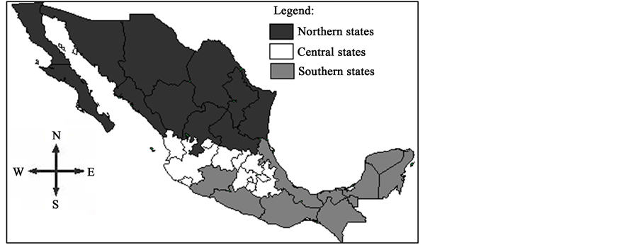
Figure 1. Mexican states and geographical regions. Source: own elaboration.
Table 3. Correlation matrix of the variables of interest.
Source: Own estimations.

Figure 2. Mexican states and regional wealth levels. Source: own elaboration.
5. Results and Analysis of the Estimates
5.1. Some Technical Details
As a consequence of the inclusion of a lagged dependent variable on the right-hand side of the equation regression,
 is a function of
 in Equation (5), then
 on the right-hand side in (5) is correlated with the error term (Baltagi [20] ). In this case, neither OLS nor fixed effects will be efficient. These dynamic regressions must be estimated through special methods, such as the general method of moments with instrumental variables. Here, a specific tool known as the two-step system GMM procedure is applied. It is suggested by Arellano and Bover [23] and Blundell and Bond [24] and revisited by Andrews and Lu [27] , which basically permits to face three implicit difficulties: serial correlation, the selection of adequate instruments and the model consistency.
Firstly, assuming that innovations follow an integrated MA(1) process, the system GMM procedure removes the cross-section fixed effects transforming each variable in the regression by means of first differences. It allows reducing the problem of serial correlation. Secondly, the GMM procedures are based on the use of instrumental variables (IV) and also help with the problem of serial correlation. However, the IV should be particularly related to the explanatory variables and at the same time they should not be correlated with the error term. Arellano and Bond [21] , Arellano and Bover [23] , Blundell and Bond [24] and Andrews and Lu [27] , among others, propose several methods with this purpose, for example applying transformations in first differences or orthogonal deviations. However, in some cases there may be a weak instruments problem, such as
 in (5), so an efficient GMM estimator is desired. For this point, several transformation options besides various sets of instrumental variables are executed. The empirical results reveal a mixture of explanatory variables in levels and lags and up to three lags of the dependent variable as instruments for equations in first differences, as a better adjustment of the model. Orthogonal deviations were no better than first differences, moreover, the estimates from the system GMM procedure by the two-step method―in accordance with Blundell and Bond [24] ―yield the best results.
Third, problems of consistency of the model and over-identifying restrictions can arise as a result of the relatively great number of temporal observations (T). In this case, the consistency and moment selection criteria are reviewed with the
 test statistic. For Arellano and Bond [28] , the
 statistic is heteroskedasticity-consistent when the two-step GMM estimator is considered. Under the null hypothesis that over-identifying restrictions are valid, the
 statistic is distributed as
 . If the null hypothesis cannot be rejected for a determined level of significance, it means that the moment conditions are acceptable.
Baltagi [20] considers that the
 statistic could have bad power when
 is large because of the great number of moment conditions that are available. However, not all the moment conditions are used. Moreover― and as Baltagi [20] suggests―the collapse option is invoked to reduce these moment conditions. In addition, Andrews and Lu [27] conclude that there is a lack of procedures to select the correct model and moment conditions in a GMM context. They consider that a trial-and-error experiment is necessary.
Finally, when two or more regressors are included in the autoregressive dynamic model, it has the disadvantage that all the dynamic marginal effects decline at the same exponential rate
 as
as
 increases. However, in this empirical essay, we do not hope that productivity responds more quickly to education than innovation or some other variable. On the contrary, the theoretical evidence highlights the reasons for the lagged response based on institutional rigidities that impede a rapid adjustment of productivity to its optimal level. Therefore, it seems reasonable to expect that the same lag structure would apply regardless of which variable causes a change in the optimal productivity. In other cases, different patterns would be expected. For example, food consumption may adjust less quickly to changes in the price of food than to changes in income. In this case, the model will not be feasible.
5.2. Results
Taking into account all the mentioned previously details, the estimates of parameters by means of the two-step system GMM procedure are summarized in Table 4. As shown, regression Equation (5) is estimated for the overall sample, three different samples according to an income-level classification and another three samples incorporating geographical criteria. Researching the consistency of the parameters by income level and geographical location is quite informative in economies such as Mexico, where the regions tend to have huge differences in both geographical and wealth contexts.
For the overall sample, the impacts on productivity are highly and statistically significant from innovation and average schooling years and weakly significant―at the 10% level―from education expenditure―see column 1 of Table 4. The estimates of average schooling years exert the greatest impact on productivity. The long-run productivity elasticities with scholarship suggest increments of productivity by 1.22% when scholarship augments by 1%, while innovation and education expenditure average smaller impacts.
Table 4. DPD results for several samples.
Notes: standard errors in parentheses. ***, ** and * indicate significance at 1%, 5% and 10%, respectively. Estimates by two-step system GMM in first differences. For all samples the instruments are levels and lags of the explanatory variables and up to three lags of the dependent variable. Source: own elaboration.
The over-identifying restrictions are valid in all samples, suggesting consistency of the model and correctly selected moment conditions.
If a regional classification according to the income level is considered―see columns 2, 3 and 4 of Table 4―it is possible to appreciate important information about the productivity of those different Mexican regions. In particular, richer states seem to base their productivity increments on innovation and scholarly performance, while in the poorer states those factors are not significant for productivity.
In the poorer states, only the education expenditure is significant. Because the regional distribution of education expenditure responds to the way in which the Mexican states are politically organized―as a federal system―it is a factor distributed as a function of population and not necessarily as a result of economic efficiency criteria; thus, the impacts tend to stand out from the factors of economic efficiency, mainly in economically lagged regions.
In addition, for the poorer sample, the relationship between average schooling years and productivity is not significant. In spite of scholarship constituting a factor that has continuously increased its performance in all the states, the non-significant result can be interpreted in the sense that increases in productivity do not correspond to increases in scholarship. A possible hypothesis is that the yields of education are not efficiently exploited because of a lack of productive structures absorbing the increasing human capital in those states. Meanwhile, in the middle-income sample, a significant relationship is observed for all the variables. Scholarly attainment is highlighted as making the major contribution to productivity.
With respect to geographical location, the estimates highlight the corresponding geographical features that differentiate the performance of the Mexican states. We can appreciate in Table 4―columns 5, 6 and 7―that the innovation is a quite important factor for the productivity of northern and central states but not for southern states. It suggests a technological gap in innovation terms in which the southern states are lagging. Notwithstanding, the yields of average schooling years on productivity are also elevated in the southern and northern states and comparatively smaller for the central states. Geographically, the education expenditure is important only in the productivity of the states belonging to the central region. Curiously, the central states make up the unique geographical region where all the variables are important contributors to their productivity. It says much about the great capacity of absorption in the productive structure of this region. This is also the case for the middle-income sample.
6. Concluding Remarks
Alluding to theoretical reasons of economic phenomena―such as the productivity―that tend to be reinforced over time, in this work dynamic panel data techniques are applied to investigate the impacts from innovation, education expenditure and average schooling years, in a regional context.
The estimated relationship among variables is compatible with the theory: the contribution on productivity varies according to the sample and the importance of the lags is confirmed. The empirical exercise highlights that effects from education and the accumulation patents have not the same intensity if the economy is rich, poor or if it belongs at the north, center or south of the country. Therefore, the design of policies must take into account this fact.
Regarding the wealth criterion, innovation stands out as the main contributor to the productivity of the richer states, but not to the poorer states. In contrast, education expenditure is very important for the productivity of the poorer, but not in the richer states. This fact has important implications for the regional economic policy. With the aim to improve the poorer states’ productivity and shorten the gap between advanced and lagged states, it seems necessary to create and promote a policy framework incentivizing intellectual property rights not only as a national action, but also as a regionally differentiated policy, in such a way that advanced technology and incentives to patent are rewarded. Nowadays, the low performance in innovation represents a restriction to growth, and at the same time the northern and central states are distancing themselves from the southern states. On the other hand, in addition to affecting the innovation technologies, for example through fomenting the establishment of foreign firms and multinationals, the university education can generate synergies to increase the innovation. Mexican states have increased the education level, but is not enough this itself action. It should be accompanied with policies that reward the higher education, for example improving the salaries of professionals.
Some limitations are also an opportunity to improve this work in the future. One of the limitations is the fact that at the state level there is not availability of variables closest to the concept of innovation and human capital, except the accumulated patents and the average schooling years. Another limitation was not including in the regression equations some control variables, such as the economy size, the weight of the high-tech industry of the states, and the spillovers arising from the neighbor states, among others. The use of such variables can affect the estimates and get a better model.
The results help to explain much of the existent inequality among the Mexican regions in terms of their productivity. These results to point out the necessity to design a regional policy directed to reduce the inequalities by creating mechanisms and conditions that allow developing the economic structure, because it is appreciated that educative improvements have not been absorbed by the economies.
References
- Becker, G. (1962) Investment in Human Capital: A Theoretical Analysis. Journal of Political Economy, 70, 9-49. http://dx.doi.org/10.1086/258724
- Schultz, T. (1963) Economic Value of Education. Columbia University Press, New York.
- Chevalier, A., Harmon, C., Walker, I. and Zhu, Y. (2004) Does Education Raise Productivity, or Just Reflect It? The Economic Journal, 114, F499-F517. http://dx.doi.org/10.1111/j.1468-0297.2004.00256.x
- Paus, E.A. (2004) Productivity Growth in Latin America: The Limits of Neoliberal Reforms. World Development, 32, 427-445. http://dx.doi.org/10.1016/j.worlddev.2003.05.002
- Power, D. and Malmberg, A. (2008) The Contribution of Universities to Innovation and Economic Development: In What Sense a Regional Problem? Cambridge Journal of Regions, Economy and Society, 1, 233-245.
- Kaldor, N. and Mirrless, J.A. (1962) A New Model of Economic Growth. The Review of Economic Studies, 29, 174- 192. http://dx.doi.org/10.2307/2295953
- Crespi, F. and Pianta, M. (2008) Demand and Innovation in Productivity Growth. International Review of Applied Economics, 22, 655-672. http://dx.doi.org/10.1080/02692170802407429
- Pencavel, J. (1991) Higher Education, Productivity, and Earnings: A Review. Journal of Economic Education, 22, 331- 359. http://dx.doi.org/10.1080/00220485.1991.10844727
- Mayhew, K. and Neely, A. (2006) Improving Productivity―Opening the Black Box. Oxford Review of Economic Policy, 22, 445-456. http://dx.doi.org/10.1093/oxrep/grj026
- Vieira, E., Neira, I. and Vázquez, E. (2011) Productivity and Innovation Economy: Comparative Analysis of European NUTS-2, 1995-2004. Regional Studies, 45, 1269-1286. http://dx.doi.org/10.1080/00343404.2010.486781
- AlAzzawi, S. (2012) Innovation, Productivity and Foreign Direct Investment-Induced R&D Spillovers. The Journal of International Trade & Economic Development, 21, 615-653. http://dx.doi.org/10.1080/09638199.2010.513056
- Harris, R., Li, Q.C. and Moffat, J. (2013) The Impact of Higher Institution-Firm Knowledge Links on Establishment- Level Productivity in British Regions. The Manchester School, 81, 143-162. http://dx.doi.org/10.1111/j.1467-9957.2011.02276.x
- German-Soto, V., Gutiérrez, L. and Tovar Montiel, S.H. (2009) Factores y relevancia geográfica del proceso de inno- vación regional en México, 1994-2006. Estudios Económicos, 24, 225-248.
- Ríos Bolívar, H. and Marroquín Arreola, J. (2013) Innovación tecnológica como mecanismopara impulsar el creci- miento económico. Evidencia regional para México. Contaduría y Administración, 58, 11-37.
- Cabral, R. and González, F.J. (2014) Gasto en investigación y desarrollo y productividad en la industria manufacturera mexicana. Estudios Económicos, 29, 27-55.
- Brown, F. and Guzmán, A. (2014) Innovation and Productivity across Mexican Manufacturing Firms. Journal of Tech- nology Management & Innovation, 9, 36-52. http://dx.doi.org/10.4067/S0718-27242014000400003
- Crespi, G. and Zuñiga, P. (2010) Innovation and Productivity: Evidence from Six Latin American Countries. IDB Working Paper Series No. IDB-WP-218.
- Mungaray, A. and Ramírez, M. (2007) Human Capital and Productivity in Microenterprises. MPRA Paper No. 4064.
- Koyck, L.M. (1954) Distributed Lags and Investment Analysis. North-Holland, Amsterdam.
- Baltagi, B.H. (2008) Econometric Analysis of Panel Data. John Wiley & Sons Ltd., Chichester.
- Arellano, M. and Bond, S. (1991) Some Tests of Specification for Panel Data: Monte Carlo Evidence and an Application to Employment Equations. Review of Economic Studies, 58, 277-297. http://dx.doi.org/10.2307/2297968
- Ahn, S.C. and Schmidt, P. (1995) Efficient Estimation of Models for Dynamic Panel Data. Journal of Econometrics, 68, 5-27. http://dx.doi.org/10.1016/0304-4076(94)01641-C
- Arellano, M. and Bover, O. (1995) Another Look at the Instrumental Variable Estimation of Error-Component Models. Journal of Econometrics, 68, 29-52. http://dx.doi.org/10.1016/0304-4076(94)01642-D
- Blundell, R. and Bond, S. (1998) Initial Conditions and Moment Restrictions in Dynamic Panel Data Models. Journal of Econometrics, 87, 115-143. http://dx.doi.org/10.1016/S0304-4076(98)00009-8
- Blundell, R. and Bond, S. (2000) GMM Estimation with Persistent Panel Data: An Application to Production Functions. Econometric Reviews, 19, 321-340. http://dx.doi.org/10.1080/07474930008800475
- Blundell, R., Bond, S. and Windmeijer, F. (2000) Estimation in Dynamic Panel Data Models: Improving on the Performance of the Standard GMM Estimator. Advances in Econometrics, 15, 53-91. http://dx.doi.org/10.1016/S0731-9053(00)15003-0
- Andrews, D.W.K. and Lu, B. (2001) Consistent Model and Moment Selection Procedures for GMM Estimation with Application to Dynamic Panel Data Models. Journal of Econometrics, 101, 123-164. http://dx.doi.org/10.1016/S0304-4076(00)00077-4
- Arellano, M. and Bond, S. (1998) Dynamic Panel Data Estimation Using DPD98 for Gauss: A Guide for Users. http://www.cemfi.es/~arellano/#dpd.
NOTES

1A political division of the Mexican states is shown in Figure 1.

2This is the Secretaría de Educación Pública (SEP) in Mexico.