Theoretical Economics Letters
Vol. 2 No. 3 (2012) , Article ID: 21518 , 4 pages DOI:10.4236/tel.2012.23050
Defining Single Asset Price Momentum in Terms of a Stochastic Process
1Korea Capital Market Institute, Seoul, Korea
2Trinity College, University of Cambridge, Cambridge, UK
3University of Sydney, Sydney, Australia
Email: *hong.jimmy@gmail.com, ses999gb@yahoo.co.uk
Received May 24, 2012; revised June 25, 2012; accepted July 26, 2012
Keywords: Momentum; Ornstein-Uhlenbeck; Price Trend; Price Autocorrelation
ABSTRACT
This paper looks at various definitions of momentum then investigates a particular definition of momentum via a statistical model where the asset price is assumed to follow a log Ornstein-Uhlenbeck process. Momentum is a term that is widely used to describe price behaviour but is not clearly defined in terms of statistical models. The results we derive show that asset price momentum is determined by price autocorrelation and that positive momentum, as commonly understood, would require explosive behaviour in log prices.
1. Introduction
Technical analysts employ many techniques in seeking profitable opportunities, one of which is the use of charts. Using charts, technical analysts seek to identify price patterns and market trends in financial markets and attempt to exploit these patterns. These patterns are often linked with the rather nebulous idea of price momentum. Much previous literature such as [1-7] explain momentum as an upward trend in a time series, which can be assets’ price, earnings or returns. But they concentrate only on historical data and do not give explanations in terms of underlying processes. [8] studies momentum in stock returns, focusing on the role of industry, size, and book-to-market factors. The paper argues that it is excess covariance, not underreaction that explains momentum in the portfolios. Again, [8] looks at cross sectional return momentum empirically without providing a technical definition of momentum. [9] measure return momentum as the change in risk premium for a percentage change in firm value, where they find that a firm’s revenues, costs, and growth options combine to determine the dynamics of its return autocorrelation and show that this insight helps momentum strategy to be profitable. Although this provides a technical definition of return momentum, it is cross sectional, not single asset momentum.
Technical analysts interpret momentum in terms of moving averages; when the current price rises above its moving average it is interpreted as an upward (bullish) trend , while a downward (bearish) trend emerges when the current price falls below its moving average. These interpretations do not really clarify if momentum is related to trend or to autocorrelation; both ideas having precise definitions in a statistical sense. We turn to the practitioner literature to see if matters are resolved. The definition of momentum in Wikipedia is “Momentum investing, also sometimes known as ‘Fair Weather Investing’, is a system of buying stocks or other securities that have had high returns over the past three to twelve months, and selling those that have had poor returns over the same period”. And in Investopedia, momentum is defined as “An investment strategy that aims to capitalize on the continuance of existing trends in the market. The momentum investor believes that large increases in the price of a security will be followed by additional gains and vice versa for declining values”.
Indeed, it is very hard to find a formal definition of price momentum that has a statistical basis. By this we mean a definition of momentum defined as a property or properties of a stochastic process. In this paper, we intend to provide a technical definition of single asset price momentum. There are two different types of momentum in terms of the number of assets involved, cross sectional momentum and single asset momentum. Unlike previous momentum literature that focuses on the relative performance of securities in the cross-section, we emphasize that this paper intends to investigate momentum within asset price process. [10] also look at a type of momentum that is similar to ours and call it “time series momentum”. This single asset momentum focuses purely on a security’s own past process. Reference [10] state the importance of the autocorrelation within a financial time series as “We find that positive auto-covariance in our futures contracts’ return drives most of the time series and crosssectional momentum effects we find in the data. Their analysis only focuses on the mean of the time series return. The contribution of the other two return components—serial cross-correlations and variation in mean returns—is small”. We are interested in price momentum instead of returns or earnings momentum because 1) most of, if not all, trading rules using technical analysis are based on past prices; and 2) the price momentum effect tends to be stronger and longer-lived than the return momentum effect. Most previous momentum studies typically include a large cross-section of stocks weighted by the previous period return.
Reference [11] defines “The Momentum Indicator is the ratio of today’s price compared to the price n periods ago: Momentum = (Close/Close n periods ago)*100. Therefore Momentum Investing is investing in securities with levels of Momentum Indicator above certain threshold.” As quoted in [12], Richard Driehaus (who is widely considered as the father of momentum investing) once said “far more money is made buying high and selling at even higher prices” (as opposed to “buy low sell high”). This Achelis’ definition of momentum has clear mathematical structure. Our main objective is that we take Achelis’ definition of momentum and investigate if it can be consistent with standard dynamic stochastic processes and, as a consequence, what will be the determinants of momentum. The obvious candidate for the asset price process is the log Ornstein-Uhlenbeck (log OU) process. The OU price process allows for serial correlation return process, which can occur for many assets. This process has been successfully used by many others including [13-15] in studying financial asset price process. The use of this process also has been heavily studied by [16]. In this paper, like [17], which show that momentum might be caused by cross autocorrelation in cross sectional stock returns, we show that autocorrelation in a single time series can also be a source of momentum.
Our main contribution is that we translate the widespread, but rather a vague, concept of momentum as a population property of a stochastic process. We investigate the definition of momentum via a statistical model of log Ornstein-Uhlenbeck process to find that 1) price momentum is determined by price autocorrelation and that 2) explosive behaviour in log prices is a necessity to relate a percentage change in the current price to a positive percentage change in the momentum measure. This association of momentum with explosive price behaviour should make practice of momentum trading of possible interest to central banks and regulators. Although our work focuses on price momentum, the same approach can be applied to other time series such as returns and earnings.
2. The Model
Whilst momentum is attributed to behavioural explanations, typically herding and conservatism bias, we shall not look at equilibrium models with momentum investors in. On the basis of previous definitions, momentum manifests itself in statistical models as possibly either trend or autocorrelation or both. Therefore we advocate the log Ornstein-Uhlenbeck model to demonstrate this. This model can be thought of as a stationary process about a trend or a random walk with drift or an explosive process about a trend. Such versatility should allow us to get some insights into the properties of momentum, as defined by Achelis. Assume that the logarithm of the asset price  has a linear trend
 . We consider the relationship

Assume a log price process,
 (1)
(1)
The solution for Equation (1) is well known,
 (2)
(2)
h is the holding period which is always positive. In this model,  can be interpreted as the degree of price autocorrelation. In fact, the model admits an exact discrete autoregressive (AR(1)) representation in which this is the autoregressive coefficient. From well-known properties of the AR(1) model, we know that stationarity and existence of a steady-state solution require
 . Indeed, we can think of two different processes for Equation (2) depending on the magnitude of the autoregressive coefficient. First, when Equation (2) is mean reverting, then
  (i.e. positive autocorrelation) and hence
 . Second, when Equation (2) is explosive, then
 , there is no stationarity nor a steady-state solution and hence
 .
.
The ratio of future price in period h to today’s price can be represented as
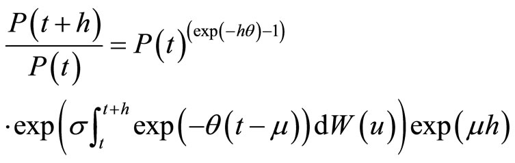 (3)
(3)
Hence the expected value of the left-hand side of Equation (3) is
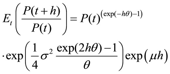 (4)
(4) This can be thought as the population momentum measure conditioned on time t. Taking logs, we get 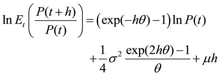 (5)
(5)
The properties of this population momentum measure can be analysed in terms of elasticities, hence the sensitivity of the Equation (4) with respect to the log of P(t). If this elasticity is positive, then there is a bullish momentum and if negative there is a bearish momentum Moreover, as elasticity, it is dimensionless, measuring the impact of a percentage change in price where impact is on a percentage change in momentum.
Proposition 1. The elasticity of the conditional population momentum with respect to the current period’s price for the log OU model can be expressed as
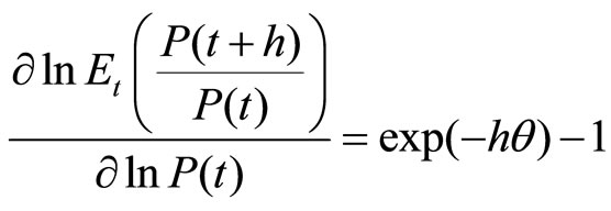 (6)
(6)
Proposition 1 clearly shows that, for log OU, momentum is about autocorrelation. Equation (6) shows that when the price process is mean reverting, the elasticity of momentum is negative while it is positive if the price is explosive. This is what we would exactly anticipate. In other words, given the high past price, the future price is low if the price process reverts around a mean but the future price is high if the price process is explosive. If we were to interpret efficient markets as a log random walk with drift, then the elasticity becomes zero. Finally, the elasticity is independent of the trend.
Proposition 2. The semi-elasticity of conditional population momentum with respect to price autocorrelation for the log OU model is
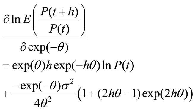 (7)
(7)
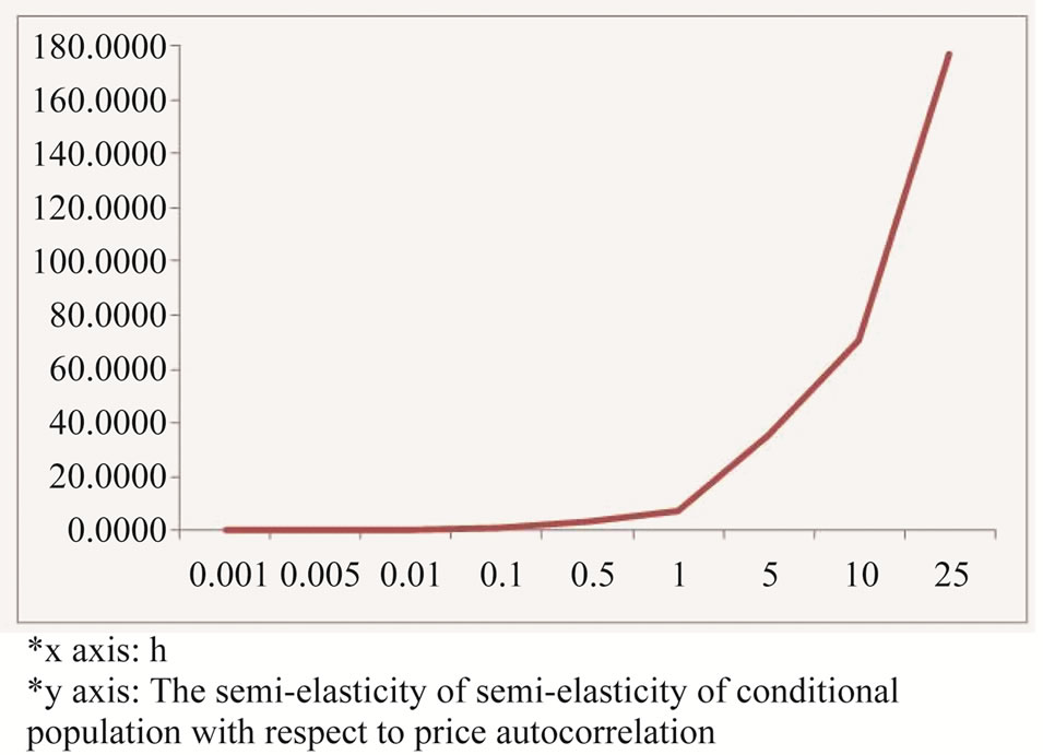
Figure 1. Equation (7) with respect to h.
We numerically investigate Equation (7) by setting the price autocorrelation 0.95. Hence 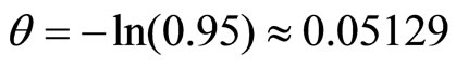 . In order to locate a sensible value of price standard deviation, we take the market standard deviation estimate of [18] as price standard deviation,
 . We take the level of S&P500 on August 15, 2011 (the most recent available data), therefore
 . We confirm that the price level and the price standard deviation are consistent since [18] estimates market standard deviation from S&P500 historical data between July 1, 2009 and July 1, 2010. We have to emphasize that there is no special reason to choose these numbers but only to locate sensible parameters.
As shown in Figure 1, the semi-elasticity of conditional population momentum with respect to price autocorrelation increases as h increases. Thus the impact of autocorrelation increases the percentage change in momentum, the longer the holding period.
3. Conclusion
In this note, we set out to translate the widespread concept of momentum as a population property of a stochastic process. We trawled the academic and practitioner to find a definition that had a meaning for a process, as opposed to a realization. Having found a definition in terms of the ratio of future prices to past/current prices, we investigate the definition of momentum via a statistical model where the price follows a log Ornstein-Uhlenbeck process. The result shows, at least in this context, that price momentum is determined by price autocorrelation, not deterministic trend, and that momentum trading would require explosive behaviour in log prices to relate a percentage change in the current price to a positive percentage change in the momentum measure. This association of momentum with explosive price behaviour makes the wide-spread practice of momentum trading of possible interest to central banks and regulators.
REFERENCES
- W. Brock, J. Lakonishok and B. LeBaron, “Simple Technical Trading Rules and the Stochastic Properties of Stock Returns,” Journal of Finance, Vol. 47, No. 5, 1992, pp. 1731-1764. doi:10.1111/j.1540-6261.1992.tb04681.x
- N. Barberis, A. Shleifer and R. Vishny, “A Model of Investor Sentiment,” Journal of Financial Economics, Vol. 49, No. 3, 1998, pp. 307-343. doi:10.1016/S0304-405X(98)00027-0
- K. G. Rouwenhorst, “International Momentum Strategies,” Journal of Finance, Vol. 53, No. 1, 1998, pp. 267- 284. doi:10.1111/0022-1082.95722
- D. Kent, D. Hirshleifer and A. Subrahmanyam, “Investor Psychology and Security Market Underand Overreactions,” Journal of Finance, Vol. 53, No. 6, 1998, pp. 1839-1886. doi:10.1111/0022-1082.00077
- H. Hong, T. Lim and J. Stein, “Bad News Travels Slowly: Size, Analyst Coverage, and the Profitability of Momentum Strategies,” Journal of Finance, Vol. 55, No. 1, 2000, pp. 265-295. doi:10.1111/0022-1082.00206
- N. Jegadeesh and S. Titman, “Profitability of Momentum Strategies: An Evaluation of Alternative Explanations,” Journal of Finance, Vol. 56, No. 2, 2001, pp. 699-720. doi:10.1111/0022-1082.00342
- W. M. Fong and L. H. Yong, “Chasing Trends: Recursive Moving Average Trading Rules and Internet Stocks,” Journal of Empirical Finance, Vol. 12, No. 1, 2005, pp. 43-76. doi:10.1016/j.jempfin.2003.07.002
- J. Lewellen, “Momentum and Autocorrelation in Stock Returns,” Review of Financial Studies, Vol. 15, 2002, pp. 533-563. doi:10.1093/rfs/15.2.533
- J. S. Sagi and M. S. Seacholes, “Firm-Specific Attributes and the Cross-Section of Momentum,” Journal of Financial Economics, Vol. 84, No. 2, 2007, pp. 389-434. doi:10.1016/j.jfineco.2006.02.002
- T. J. Moskowitz, Y. H. Ooi and L. H. Pedersen, “Time Series Momentum,” Journal of Financial Economics, vol. 104, No. 2, 2012, pp. 228-250. doi:10.1016/j.jfineco.2011.11.003
- S. Achelis, “Technical Analysis from A to Z,” 2nd Edition, McGraw-Hill Companies, New York, 2000.
- J. D. Schwager, “The New Market Wizards: Conversation with America’s Top Traders,” HarperCollins, New York, 1992.
- A. Lo and J. Wang, “Implementing Option Pricing Models When Asset Returns Are Predictable,” Journal of Finance, Vol. 50, No. 1, 1995, pp. 87-129. doi:10.1111/j.1540-6261.1995.tb05168.x
- R. Kramer and M. Richter, “A Generalized Bivariate Ornstein-Uhlenbeck Model for Financial Assets,” Tagungsband zum Workshop “Stochastische Analysis”, Chemnitz, 2007.
- O. Onalan, “Financial Modelling with Ornstein-Uhlenbeck Processes Driven by Levy Process,” Proceedings of the World Congress on Engineering, London, Vol. 2, 1-3 July 2009.
- A. R. Bergstrom, “Continuous Time Econometrics Modelling,” Oxford University Press, Oxford, 1990
- A. Lo and A. C. MacKinlay, “When Are Contrarian Profits Due to Stock Market Overreaction?” Review of Financial Studies, Vol. 3, No. 2, 1990, pp. 175-205. doi:10.1093/rfs/3.2.175
- K. J. Hong and S. Satchell, “The Sensitivity of Beta to the Time Horizon When Log Prices Follow an OrnsteinUhlenbeck Process,” European Journal of Finance, 2012, in Press. doi:10.1080/1351847X.2012.698992
NOTES
*Corresponding author.