Journal of Mathematical Finance
Vol.3 No.4(2013), Article ID:39621,11 pages DOI:10.4236/jmf.2013.34048
Is the Driving Force of a Continuous Process a Brownian Motion or Fractional Brownian Motion?
1School of Management, Fudan University, Shanghai, China
2Department of Mathematics, Hong Kong University of Science and Technology, Hong Kong, China
3School of Mathematics and Statistics, Lanzhou University, Lanzhou, China
Email: kongxblqh@gmail.com, majing@ust.hk, *licuixia@lzu.edu.cn
Copyright © 2013 Xinbing Kong et al. This is an open access article distributed under the Creative Commons Attribution License, which permits unrestricted use, distribution, and reproduction in any medium, provided the original work is properly cited.
Received August 9, 2013; revised September 21, 2013; accepted October 8, 2013
Keywords: Itô semimartingale; Fractional Brownian motion
ABSTRACT
Itô’s semimartingale driven by a Brownian motion is typically used in modeling the asset prices, interest rates and exchange rates, and so on. However, the assumption of Brownian motion as a driving force of the underlying asset price processes is rarely contested in practice. This naturally raises the question of whether this assumption is really appropriate. In the paper we propose a statistical test to answer the above question using high frequency data. The test can be used to validate the assumption of semimartingale framework and test for the existence of the long run dependence captured by the fractional Brownian motion in a parsimonious way. Asymptotic properties of the test statistics are investigated. Simulations justify the performance of the test. Real data sets are also analyzed.
1. Introduction
There has been extensive literature in using Itô's semimartingale driven by a Brownian motion to model the asset prices, interest rates and exchange rates, since the seminal work by [1-3]. Statistical inference of Itô's semimartingales is also investigated by many authors, including [4-7] among others.
However, the assumption of Brownian motion as a driving force of the underlying asset price processes is rarely contested statistically. This naturally raises the question of whether this assumption is really appropriate. If not, what alternative can one use in place of Brownian motion? In this paper, we will focus on the use of more general fractional Brownian motion as a driving force if the usual Brownian motion is not appropriate.
The failure of models based on (conditional) uncorrelated increments to describe certain financial data sets has been observed since [8]and [9]. In their works, significant long run dependence was found. To take the long run dependence into account in modeling financial data, [10] proposed to replace Brownian motion with fractional Brownian motion. Using Wavelet method, [11] studied the fractal dimension of the S&P 500 data sampled every minute. They found empirically that the Hurst parameter of the S&P 500 data was significantly above the efficient market value  and began to approach that level around 1997. They attributed the trend to the increase in internet trading. [12] investigated the theoretical variational properties of continuous-time processes driven by a fractional Brownian motion using high frequency data.
Before moving on, we define a fractional Brownian motion with Hurst parameter , which is given by
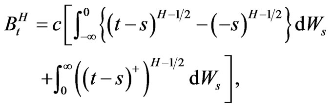 (1)
(1)
for , where
  is a standard Brownian motion with
 ,
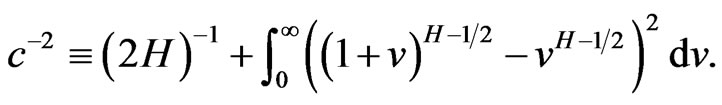
,  and
and  are the positive and negative parts of
 , and
, and
Note that  reduces to a standard Brownian motion when
 , and otherwise
  becomes a selfsimilar process with (long run) dependence when
 ; the latter property is very attractive in financial models.
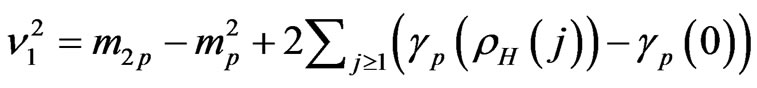
The purpose of this paper is to develop some tests to see whether the driving force is a Brownian motion or a true fractional Brownian motion. In terms of the Hurst parameter, this can be formulated as
 (2)
(2)
We introduce a method to test (2) based on the asymptotic normality of the ratio of two realized power variations with different sampling frequencies.
If a test rejects , then a fractional Brownian motion will be used in modeling. One problem of using the integral process driven by a fractional Brownian motion is the admission of arbitrage when the integral is defined in a pathwise Stieltjes way, in [13]. The theory of modeling using fractional Brwonian motion was renewed after the work of [14] in which a new type of integration based on the Wick product was introduced. If the new Wick type integration is adopted, [15] proved that the fractional Black-Scholes market has no arbitrage opportunities. However, it is hard to give economic interpretations to trading strategies using the Wick type integration, in [11]. In [11,] the pathwise Stieltjes integration was suggested although arbitrage opportunities of [13]’s type exist. They argued that strategies to make gains with no risk involve exploiting the very fine-scale properties of the process’ trajectories. The ability of a trader to implement this type of strategy is likely to be hindered by market frictions, such as transaction costs and minimum amount of time between two consecutive transactions. Indeed [16] showed that by introducing a minimal amount of time between two consecutive transactions, arbitrage opportunities are ruled out from a geometrical fractional Brownian motion.
In this paper, we will implement the pathwise Stieltjes integration that has good interpretations in defining a self-financing strategy. Using high frequency data, our test could give insight into 1) whether the underlying dynamic shows long run dependence; 2) whether the underlying dynamic is a semimartingale; and 3) how rough is the underlying dynamics in terms of its Hurst parameter, e.g., is it ?
?
The paper is organized as follows. In Section 2, we give some preliminaries and assumptions. Test statistic is given in Section 3. Main results are also presented in Section 3. Simulations are run in Section 4. Section 5 is devoted to real data analysis. Section 6 discusses some future problems. Technical proofs are postponed to the Appendices.
We assume that the observations are
 ,
, .
.
For simplicity, we further assume that
are equally spaced, that is,
 .
.
we denote the ith one-step increment by
 .
.
Mathematically, high frequency data set means that  for fixed
 . Although in theory we will consider the limiting case where
 , in practice
  is strictly positive but close to 0.
2. Preliminaries and Assumptions
2.1. Properties of Fractional Brownian Motion
Throughout this paper, we define  as the natural filtration of
  for
for , and
, and . The
. The  given in (1) has the following useful properties:
• It is a semimartingale only if .
.
• It is a zero-mean Gaussian process with
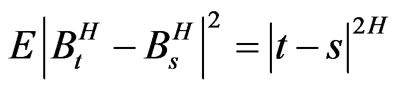
and
 .
.
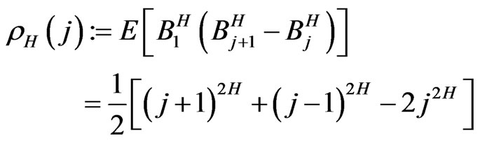
• For ,
,  is a stationary series.
•  is
is  -Hölder continuous for any
 . Hence
  has finite
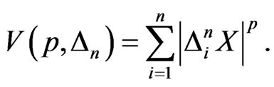
  th-variation where the qth-variation of a process
  is defined as
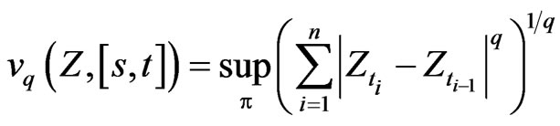
where the supremum is taken over all partition  of
of .
.
Let  be a positive process adapted to
 , the integral process,
  be defined as the pathwise Riemann-Stieltjes integral. By Young's inequality, c.f. [12], the discretization error of the integral process could be controlled by
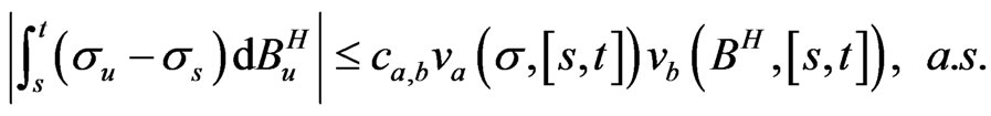 (3)
(3)
where
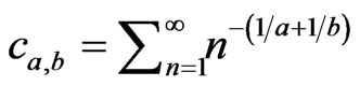 .
.
So to make the right side of (3) finite,  , i.e.,
  could at most have finite
  th power variation.
2.2. Model Assumptions
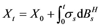
As studied in [12], [17] and the references therein, we assume that the model is a simple continuous process of the following integral form
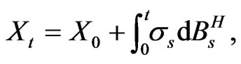 (4)
(4)
where  is the initial value. We make the following assumptions on the diffusive coefficients.
Assumption 1:  is a locally bounded càdlàg processes.
Assumption 2:  is an
is an  -Hölder continuous process with
 .
.
3. Test Statistics
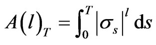
Our test is based on power variational property of :
:
Under Assumptions 1-2, it can be shown
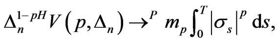 (5)
(5)
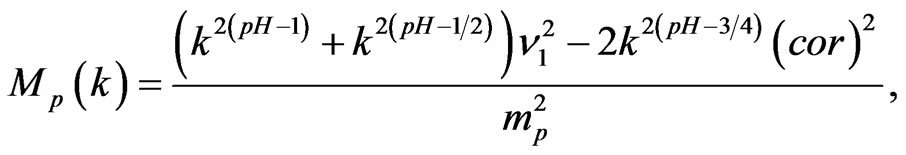
where  is some constant depending only on
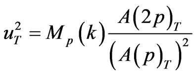
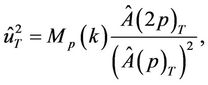
 . Since the right side of (5) is unknown, one could use the two-time scale technique as used in [18] to define the test statistic as follows,
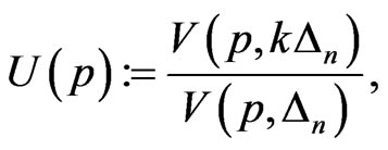 (6)
(6)
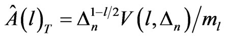
where
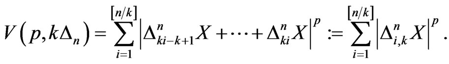
(7)
It is worthy of noticing that [4] proposed a test statistic of the same form as (6) in the context of testing for the presence of jumps within the semi-martingale framework.
Now we state our main results.
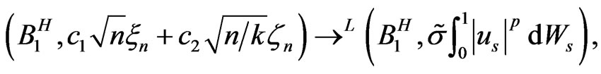
Theorem 1: Under Assumptions 1-2, we have 1) 2) if
2) if  and
and ,
,
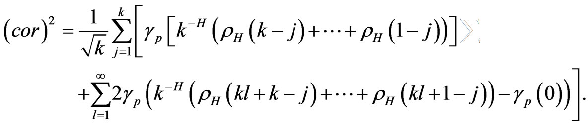
where  is a centered Gaussian random variable conditional on
  with the conditional variance
 where
where
and
where
 ,
,
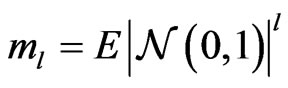
where
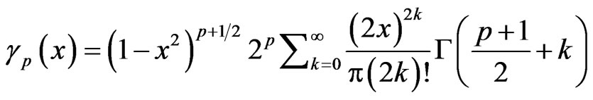
with  be the Gamma function, and
  is a constant dependent on
 .
.
Remark 1
• Under , the condition
  could be weakened, actually,
  could be semimartingales driven by Brownian motion where paths of
  are
are
 -Hölder continuous, c.f. [19].
• From Part 1 of Theorem 1, an estimator of  can be given by
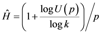 .
.
The behavior of  depends on
 , and so can be used as a test statistic. From the above theorem,
  is asymptotically normal with unknown conditional variance
  under
under . By (5), a consistent estimator of
  under
under  is
is
where
 .
.
From Theorem 1, we reject  if
if
where  satisfies
 .
.
By Theorem 1 and (5), we have
Theorem 2: Under the assumptions in Part 2 of Theorem 1, we have
and
 .
.
Therefore, our test is of asymptotic size  with asymptotic power one.
4. Simulation Studies
4.1. Assessment of the Size
In assessing the performance of the size of the test, we draw 5000 samples of size  from the following stochastic volatility process driven by a Brownian motion
with
and . We take
 ,
,  ,
,  ,
, . Set the time horizon to be
  (day) consisting of 6.5 trading hours.
We use two different sample sizes, . Figure 1 shows the histograms of the test statistics under
 . The histograms imply that the normal approximation matches well the sampling distribution of the test statistics
  under
under .
.
Take the nominal level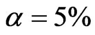 . The dot-dashed
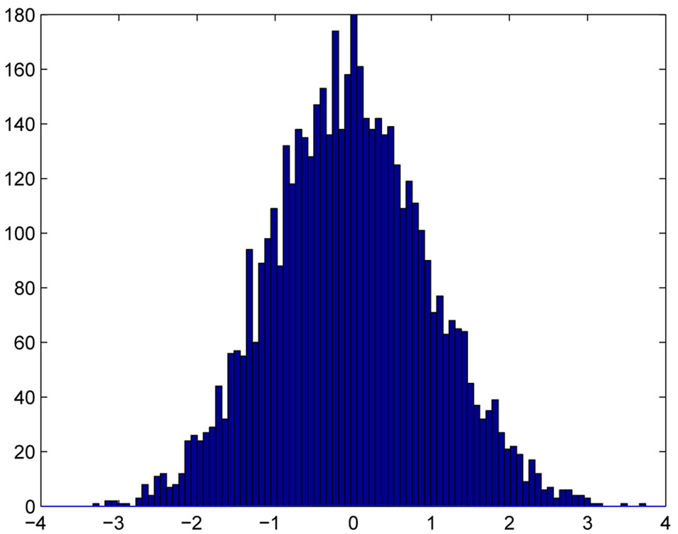
Figure 1. Histograms of the test statistics under :
:  in the left panels;
  in the right panels.
curve in Figure 2 gives the empirical sizes of the test based on  against
  when
when , from which we see that the type I error probabilities are well controlled.
4.2. Assessment of the Power
We simulate only the geometric fractional Brownian motion for 5000 times, c.f. [20], i.e.,
where  and
and  are two constants. We take
  and
and  around
 , in order to be comparable to the data generating process used in the assessment of the size. We set
 . The simulations when
  was also done but will not be listed here to save space. The conclusions are the same as those given below.
Table 1 gives the averaged  over 5000 repetitions. From the table, whatever the values of
  and
and , they are very close to
  and here
 ,
, . Table 2 reports the empirical power of the test based on
 . We make the following remarks.
• The powers are insensitive to different values of  's.
's.
• The powers grow bigger as  moves away from
 , and the test is very powerful especially when
 .
.
5. Real Data Analysis
We now implement our test to some real data sets. The first three data sets are from the New York Stock Exchange. Another two data sets, SZ000002 and SH000001, are from the Shenzhen Stock Exchange and Shanghai Stock Exchange of China, respectively.
We use the stock price records of Microsoft (MSFT) in the trading days: Nov. 1, and Dec. 1., 2000, and that of Dell Company (DELL) in Dec. 1, 2011. All data sets are from the TAQ database. For prices recorded simultaneously, we use the average. To weaken the po-ssi-ble effect from microstructure noise, we sparsely sample observations and the sample sizes for the aforementioned three trading days are 448, 568 and 528, respectively. If i.i.d. microstructure noises are assumed, then the microstructure noise would drive  to
to  as
as 
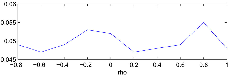
Figure 2. Empirical sizes of the test based on  against
 .
.
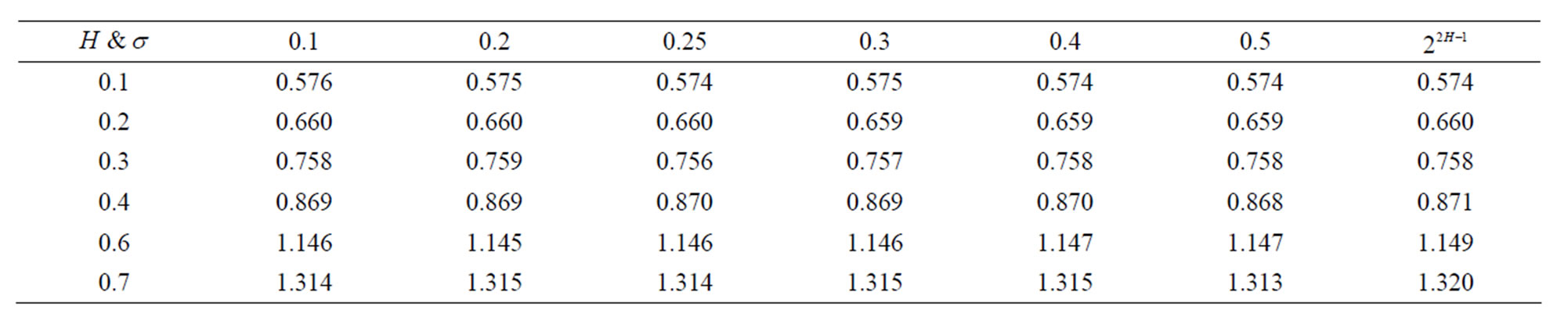
Table 1. Averaged  over different
  and
and .
.
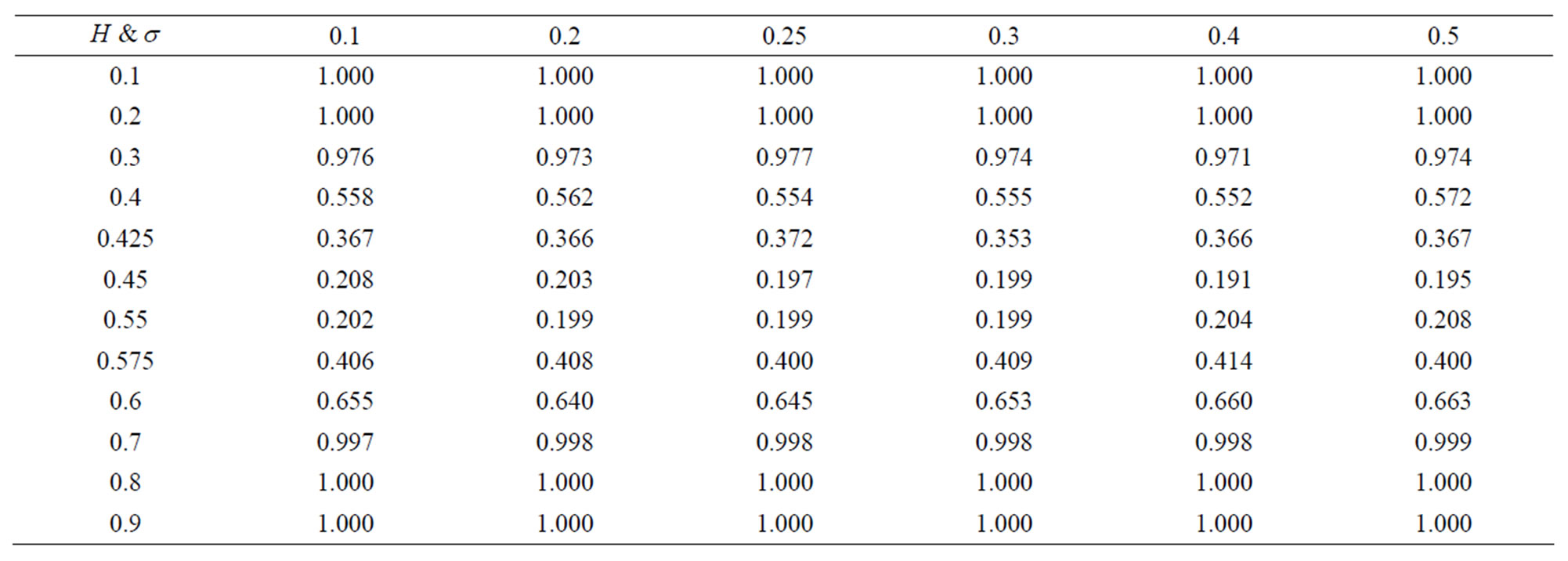
Table 2. Empirical powers of the test based on  over different
  and
and .
.
if . The results shown later demonstrate that the sparse sampling is effective since all estimated
  of all real data sets are away from
 . Finally, we take logarithm of the sparsely sampled prices and use the log prices to calculate the test statistics. We set
  (day) consisting of 6.5 hours of trading time.
The test statistics and an estimate of the Hurst parameter are provided in Table 3. U(2) is given in (3.5) with p = 2, its studentized form is given by t. Seen from the table, our test do not reject the use of Brownian motion as the driving force for all three data sets at the significance level of 5%.
Next, we analyze the stock price records of SZ000002 and SH000001. Prices are recorded from 9:25 am - 15:00 pm in the trading day Jan. 1, 2004. Figure 3 displays the log prices against the time. An obvious dependence structure among returns is observed in both plots which demonstrates strong dependence between (log) returns.
Test statistics and estimates of the Hurst parameters of the log price dynamics of these two stocks are given in Table 4. The sample sizes of SZ000002 and SH000001 are respectively 356 and 394. Seen from Table 4, we have the following observations:
• Although we do not reject  for SZ000002, minor evidences of the departure of the driving force from the Brownian motion are seen.
• Strong evidence against the Brownian motion as the driving force are shown for SH000001.
• In contrast to Table 3, it looks that the dynamics of the two Chinese stocks deviate from semimartingales driven by the Brownian motion much while semimartingales driven by the Brownian motion are still good approximation to the three U.S. stocks. This is in fact to be expected since the New York Stock Exchange is a far more efficient market than the Shenzhen Stock Exchange and Shanghai Stock Exchange.
6. Discussions
In this paper, we develop test to check whether the driving force of continuous integral processes with drift is a Brownian motion or a fractional Brownian motion. There is little literature in this direction, and there are some interesting future research directions. Here are a couple of examples.
1) It is commonly accepted that jumps exist in price processes, which has been well studied in the literature. So it is of interest to extend our results to process with jump components. Here, the truncated power variation as in [21], should prove useful, and the results in this paper may still hold true for appropriate choice of .
.
2) The effect of the microstructure noise to the test statistics will also be investigated in the future work.
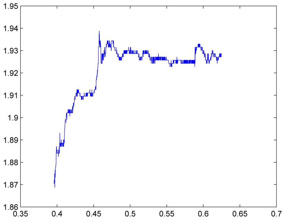
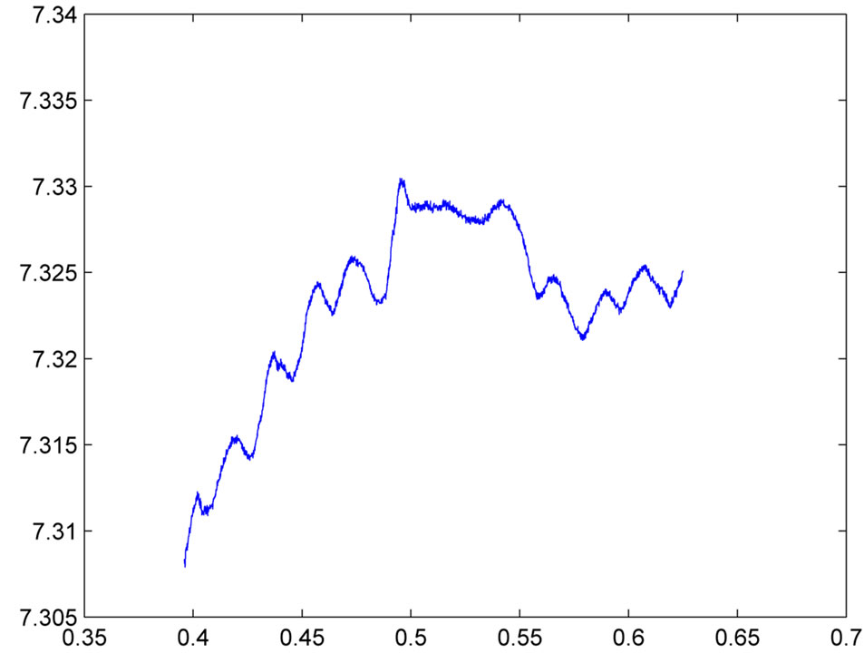
Figure 3. Plots of the Prices of SZ000002 (left panel) and SH000001 (right panel) against Time.
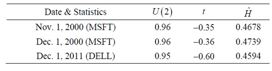
Table 3. Test Statistics and Estimate of the Hurst Parameter.
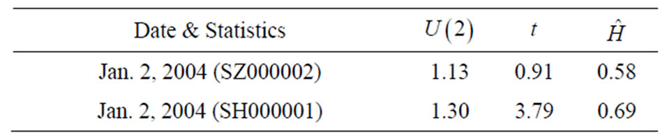
Table 4. Test Statistics and Estimate of the Hurst Parameter,  (SZ000002) and
  (SH000001).
Asymptotically, the microstructure noise would drive  to
to . Multi scale technique or pre-averaging method would serve as good ways to eliminate the effect of the microstructure noise first, c.f. [18] and [22]. Many theoretical works and practical analyses can be done along this line.
5. Acknowledgements
The authors would like to thank the editor, an associate editor and referees for their constructive suggestions that improved this paper considerably. Kong’s work is supported in part by the NSF China (11201080) and the Humanity and Social Science Youth Foundation of Chinese Ministry of Education (12YJC910003), and in part by the Fundamental Research Funds for the Central Universities
(FDU20520133198). Jing’s research is supported by Hong Kong RGC Grants HKUST6019/10P, HKUST- 6019/12P, HKUST6022/13P, and in part by the Fun-14 damental Research Funds for the Central Universities, Research Funds of Renmin University of China (Grant no. 10XNL007), and by NSF China (Grant no. 71071010). Li’s work is supported by the NSF China (11301236) and the Fundamental Research Funds for the Central Universities (lzujbky-2012-179), and in part by the NSF China (41271038).
REFERENCES
- F. Black and M. Scholes, “The Pricing of Options and Corporate Liabilities,” Journal of Political Economy, Vol. 81, No. 3, 1973, pp. 133-155.
- J. Hull and A. White, “Pricing Interest Rate Derivative Securities,” Review of Financial Studies, Vol. 3, No. 4, 1990, pp. 573-592. http://dx.doi.org/10.1093/rfs/3.4.573
- S. Heston, “A Closed-From Solution for Options with Stochastic Volatility with Applications to Bond and Currency Options,” Review of Financial Studies, Vol. 6, No. 2, 1993, pp. 327-343. http://dx.doi.org/10.1093/rfs/6.2.327
- Y. Aït-Sahalia and J. Jacod, “Testing for Jumps in a Discretely Observed Process,” The Annals of Statistics, Vol. 37, No. 1, 2009, pp. 184-222. http://dx.doi.org/10.1214/07-AOS568
- Y. Aït-Sahalia and J. Jacod, “Is Brownian Motion Necessary to Model High Frequency Data?” The Annals of Statistics, Vol. 38, No. 5, 2010, pp. 3093-3128. http://dx.doi.org/10.1214/09-AOS749
- O. E. Barndorff-Nielsen and N. Shephard, “Econometrics of Testing for Jumps in Financial Economics Using Bipower Variation,” Journal of Financial Econometrics, Vol. 2, No. 1, 2006, pp. 1-48. http://dx.doi.org/10.1093/jjfinec/nbh001
- V. Todorov and G. Tanchen, “Activity Signature Functions for High-Frequency Data Analysis,” Journal of Econometrics, Vol. 154, No. 2, 2010, pp. 125-138. http://dx.doi.org/10.1016/j.jeconom.2009.06.009
- M. T. Greene and B. D. Fielitz, “Long term Dependence in Common Stock Returns,” Journal of Financial Economics, Vol. 4, No. 3, 1977, pp. 339-349. http://dx.doi.org/10.1016/0304-405X(77)90006-X
- B. B. Mandelbrot, “When Can Price Be Arbitraged Efficiently? A Limit to the Validity of the Random Walk and Martingale Models,” Review of Economic Statistics, Vol. 53, No. 3, 1971, pp. 225-236. http://dx.doi.org/10.2307/1937966
- N. J. Cutland, P. E. Kopp and W. Willinger, “Stock Price Returns and the Joseph Effect: A Fractal Version of the Black-Scholes Model,” Progress in Probability, Vol. 36, 1995, pp. 327-351.
- E. Bayraktar, H. V. Poor and R. Sircar, “Estimating the fractal Dimension of the S&P 500 Index Using Wavelet Analysis,” International Journal of Theoretical and Applied Finance, Vol. 7, No. 5, 2004, pp. 615-643. http://dx.doi.org/10.1142/S021902490400258X
- J. Corcuera, D. Nualart and J. Woerner, “Power Variation of Some Integral Fractional Processes,” Bernoulli, Vol. 12, No. 4, 2006, pp. 713-735. http://dx.doi.org/10.3150/bj/1155735933
- L. Rogers, “Arbitrage with Fractional Brownian Motion,” Mathematical Finance, Vol. 7, No. 1, 1997, pp. 95-105. http://dx.doi.org/10.1111/1467-9965.00025
- T. E. Duncan, Y. Hu and B. Pasik-Duncan, “Stochastic Calculus for Fractional Brownian Motion,” SIAM Journal on Control and Optimization, Vol. 38, No. 1, 2000, pp. 582- 612.
- B. Oksendal and Y. Hu, “Fractional White Noise and Applications to Finance,” Infinite Dimensional Analysis, Quantum Probability and Related Topics, Vol. 6, No. 1, 2000, pp. 1-32.
- P. Cheridito, “Arbitrage in Fractional Brownian Motion Models,” Finance and Stochastics, Vol. 7, No. 4, 2003, pp. 533-553. http://dx.doi.org/10.1007/s007800300101
- S. Si, “Two-Step Variations for Processes Driven by Fractional Brownian Motion with Applications in Testing for Jumps form the High Frequency Data,” Ph.D. Thesis, University of Tennessee, Knoxville, 2009.
- L. Zhang, P. A. Mykland and Y. Ait-Sahalia, “A Tale of Two Time Scales: Determining Integrated Volatility with Noisy High-Frequency Data,” Journal of the American Statistical Association, Vol. 100, No. 472, 2005, pp. 1394-1411. http://dx.doi.org/10.1198/016214505000000169
- O. E. Barndorff-Nielsen, S. Graversen, J. Jacod and N. Shephard, “A Central Limit Theorem for Realized Power and Bipower Variations of Continuous Semi Martingales,” From Stochastic Calculus to Mathematics, 2006, pp. 33-68.
- D. Nualart, “Stochastic Calculus with Respect to the Fractional Brownian Motion and Applications,” Contemporary Mathematics, Vol. 336, 2003, pp. 3-39. http://dx.doi.org/10.1090/conm/336/06025
- C. Mancini, “Estimating the Integrated Volatility in Stochastic Volatility Models with Lévy Type Jumps,” Technical Report, University di Firenze, Firenze, 2004.
- J. Jacod, Y. Li, P. A. Mykland, M. Podolskij and M. Vetter, “Microstructure Noise in the Continuous Case: The Pre-Averaging Approach,” Stochastic Processes and Their Applications, Vol. 119, No. 7, 2009, pp. 2249-2276. http://dx.doi.org/10.1016/j.spa.2008.11.004
Appendix A: Proofs of Main Theorems
By the standard localization method, it suffices to prove the main results under the following strengthened assumptions.
Assumption 3:  is a bounded process.
In the sequel,  will stand for a constant that may take different values at different appearance.
Proof of Theorem 1 Let
Simple algebras yield
Then Theorem 1 is a straightforward consequence of Proposition 1 of which the proof is given later in Appendix B.
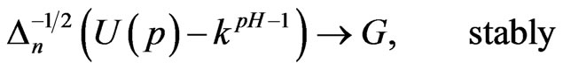
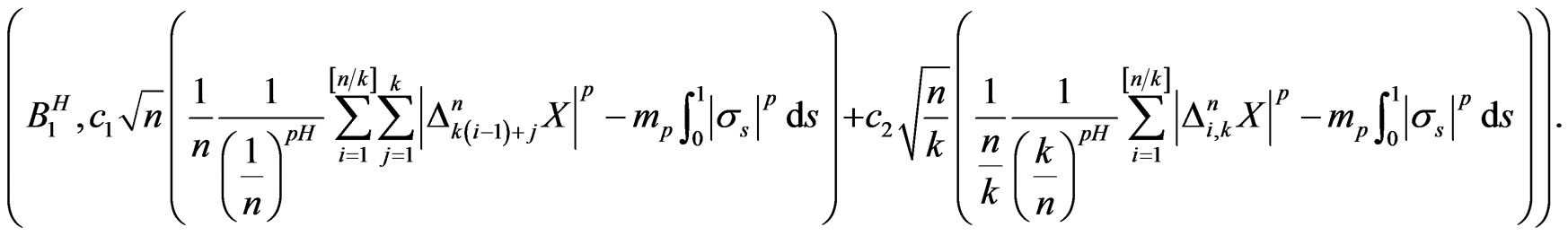
Proposition 1: Under Assumptions 1-3, if ,
,  and
and , then we have
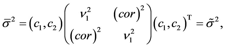
stably, where  is a centered bivariate Gaussian random vector conditional on
  with
with
 ,
,
 ,
, .
.
Proof of Theorem 2 The first convergence is a consequence of Theorem 1. Now we prove the second convergence. Under ,
,
and . Therefore we further have
and . By the rejection rule, the second convergence is proved.
Appendix B: Proof of Proposition 1
To prove Proposition 1, we need the following lemma.
Lemma 1
Proof. For simple, denote
and
 .
.
Then, we have
 ,
,  and
and
Then,
Now, for , we have
when we fixed ,
,  , then we have
Proof of Proposition 1: Recall that
 .
.
For simplicity, we assume that  which implies that
 . Then by the extended Wold device, see e.g. Lemma 4.32 in [17], it suffices to show that for any
 ,
,
 (8)
(8)
where,
 .
.
Rewrite the left side of (8) as
For any  we write
and
where
 and
and 
 with
with 
Then the left side of (8) is equal to

From the proof of Theorem 4 in [12], we know that all terms are negligible in probability except for
where,
From Lemma 1, we have for fixed , as a vector,
stably as , where
So, we have that for any  -measurable random variables,
 ,
,  as
as ,
,
where W is a Brownian motion independent of . Hence,
stably, as m tends to infinity. On the other hand,
converges uniformly in probability to  as n tends to infinity. This implies, by letting first m and then n tend to infinity, that
converges in distribution to

stably.
Note that
which completes the proof of (8).
NOTES
*Corresponding author.