ABSTRACT

The risk-sensitive asset management problem with a finite horizon is studied under a financial market model having a Wishart autoregressive stochastic factor, which is positive-definite symmetric matrix-valued. This financial market model has the following interesting features: 1) it describes the stochasticity of the market covariance structure, interest rates, and the risk premium of the risky assets; and 2) it admits the explicit representations of the solution to the risk-sensitive asset management problem.

1. Introduction

1.1. Risk-Sensitive Asset Management

Consider a continuous-time financial market that consists of one riskless asset and risky assets. The price process of the riskless asset and that of the

risky assets, , where

denotes the transpose of a vector or matrix, are semimartingales defined on a filtered probability space. Define the wealth process of a self-financing investor governed by the following stochastic differential equation (SDE):

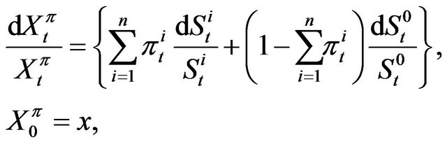(1.1)

where is the initial wealth of the investor, and, is the dynamic investment strategy of the investor. Let

(1.2)

be the growth rate of the wealth at time. For given constants and, define the risksensitized expected value of by

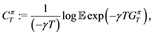
which is rewritten as

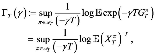
and interpreted as the certainty equivalent value of with respect to the exponential criterion function. We are interested in maximizing, that is,

(1.3)

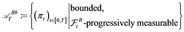
which we call the risk-sensitive asset management problem. Here, is a space of admissible investment strategies and is a subset of, the totality of -dimensional -progressively measurable processes

on the time interval such that almost surely.

Remark 1.1 The risk-sensitive asset management problem (1.3) has been well-studied under a linear-Gaussian market model, for example, by [1-7]. In those works, the price processes are given by the solutions to the following system of SDEs:

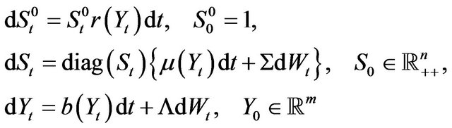(1.4)

on a filtered probability space endowed with the -dimensional -Brownian motion,. Here, denotes the diagonal matrix whose th element is equal to the th element of, , , and

(1.5)

with, , , , , , and. We reformulate (1.3) with (1.1), (1.2), (1.4), and (1.5) as a linear exponential quadratic Gaussian stochastic control problem, and the optimal investment strategy (portfolio)

for (1.3) is represented explicitly:

Here, is the solution to a matrix differential Riccati equation, and is the solution to a linear differential equation, including.

Remark 1.2 Intuitively, recalling the cumulant expansion,

where denotes variance, we interpret (1.3) as a risk-sensitized optimization of the expected growth rate maximization,

1.2. Wishart Factor Model

The main aim of the present paper is to introduce a simple and tractable market model that satisfies the following requirements:

• The model describes the stochasticity of the covariance structure of, interest rates, and mean-return rates of.

• The model admits an explicit representation of the optimal investment strategy for (1.3).

For the purpose, we employ a Wishart autoregressive process as a stochastic factor, which is positive-definite symmetric matrix-valued. Such matrix-valued processes have been introduced and studied by [8], and recently, generalizations have been intensively studied, for example, see [9,10], and the references therein. Moreover, these processes are now extensively utilized for financial modeling. We can refer to the examples given below.

• Modeling of multivariate stochastic volatility (covariance) under the risk-neutral probability: see [11-16].

• Modeling of multivariate asset price process under physical probability with stochastic covariance and mean-return rates: see [14,17,18].

• Modeling of (term structure of) interest rates and stochastic intensity for credit risk: see [14,17,19,20].

Our market model defined by (2.1)-(2.4) in Section 2 is an extension of the model employed by [18], (see Example 2.1), who studied the expected CRRA-utility ma ximization of terminal wealth, which is essentially equivalent to (1.3). A main contribution of the present paper is a rigorous mathematical analysis of portfolio optimization problem (1.3) under a flexible Wishart autoregressive stochastic factor model: We strengthen the mathematical results in [18] by formulating an appropriate space of admissible trading strategies (see (3.5)) and showing a verification theorem for the candidate of the optimal strategy (see Theorem 3.1), both of which are omitted in [18].

In the next section, we introduce our market model with a Wishart autoregressive factor and present preliminary calculations of the associated Hamilton-JacobiBellman (HJB) equation for solving risk-sensitive asset management problem (1.3). In Section 3, we introduce our main results. In Section 4, we show the proof of the main theorem after preparing lemmas.

2. Setup

2.1. Market Model with Wishart Autoregressive Factor

Let be a filtered probability space endowed with the -dimensional -Brownian motion, , and the

-dimensional -Brownian motion,

, which is independent of. Using a constant vector so that, we define another -dimensional Brownian motion

, by

which is correlated with as

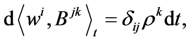
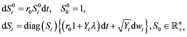
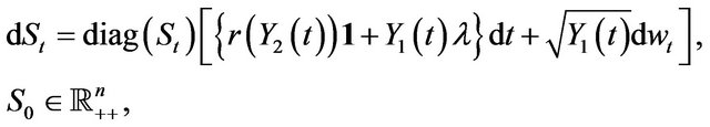
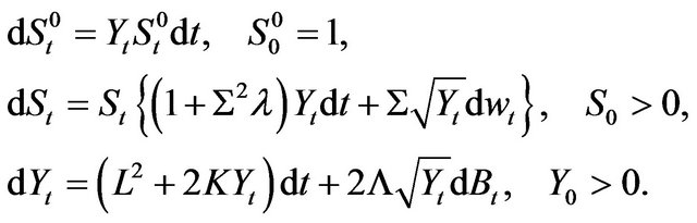
where denotes the quadratic covariation, and denotes Kronecker’s delta. We consider the price processes, described by the following system of SDEs:

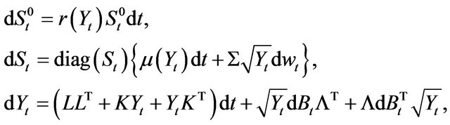(2.1)

with the initial values, and. Here, we denote by the totality of -dimensional, real, symmetric matrices, and. Furthermore, for, we define

(2.2)

where, , and. Also, we assume that is full rank, that is,

(2.3)

We also assume that, and that satisfies

(2.4)

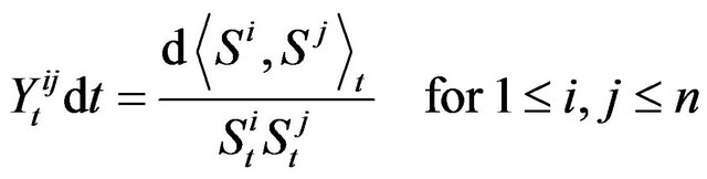
Condition (2.4) ensures almost everywhere on, which was established by Mayerhofer et al. (2011) using a generalized form of SDE, including a jump martingale part. The -valued process is a stochastic factor process, which linearly depends on the covariance structure of as

(2.5)

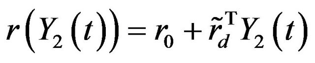
as well as on the interest rate

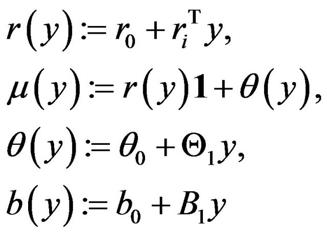
(2.6)

and on the so-called risk premium of,

(2.7)

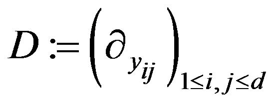
Remark 2.1 From (2.6), we see that the interest rate process is included in the so-called affine class: is an affine function of and the process, whose infinitesimal generator is given by

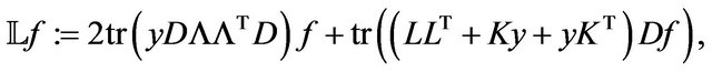(2.8)

where and

(2.9)

is indeed an affine diffusion. To review affine processes and their financial applications, see, for example, [21], [22], and the references therein.

Remark 2.2 The condition (2.7) on the structure of the risk-premium vector is rewritten as

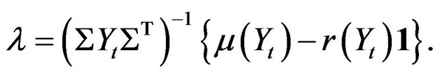
So we interpret that the so-called mean-variance term in portfolio optimization theory is assumed to be constant.

The following are concrete examples of setting up (2.1) and (2.2).

Example 2.1 (Stochastic Covariance) Let

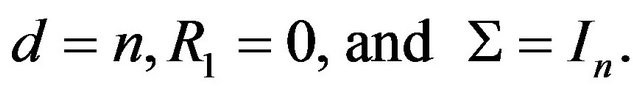
Concretely, we have

with the third equation in (2.1). describes the infinitesimal covariance and the risk premium of as

and

This is exactly the model employed in Section 1 of [18] to study expected CRRA-utility maximization of terminal wealth.

Example 2.2 (Stochastic Covariance and Interest Rate) We present a slight generalization of Example 2.1 to include stochasticity of interest rates. Let

where we set if. Then, letting

and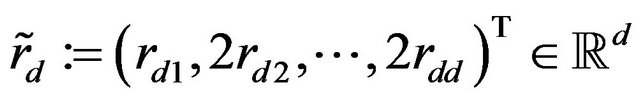, we see that

is the risk-free interest rate with the latent factor and that

where describes the infinitesimal covariance and the risk premium of as

and

Example 2.3 (Cox-Ingersoll-Ross Interest Rate Factor) Let

Then, we see

This financial market model with Cox-Ingersoll-Ross’s interest rate is treated in [23] to study (1.3).

Under the financial market model comprising (2.1) and (2.2) with the assumptions (2.3) and (2.4), we are interested in treating the risk-sensitive asset management problem (1.3).

2.2. Deriving the HJB Equation

To tackle (1.3), we employ a dynamic programming approach: Recall that wealth process (1.1) of a selffinancing investor, combined with (2.1), is rewritten as

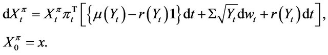
So, we see

where we set

(2.10)

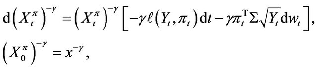
Hence, we have

where we define

(2.11)

Let

For, we define the probability measure on by the formula

By Cameron-Martin-Maruyama-Girsanov’s theorem, we see that the -valued process, defined by

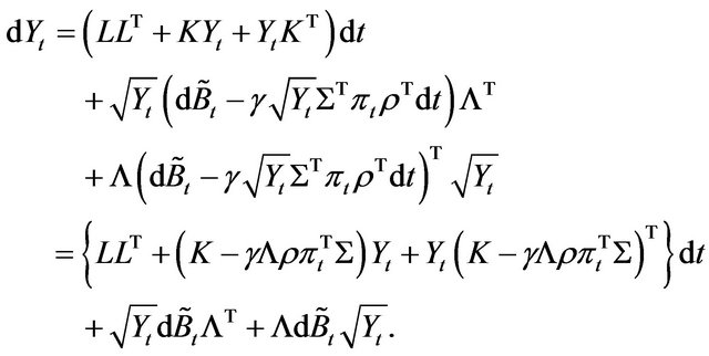
is a -Brownian motion. Moreover, we see that has the -dynamics

Recall that, for, we have

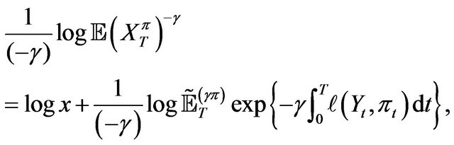(2.12)

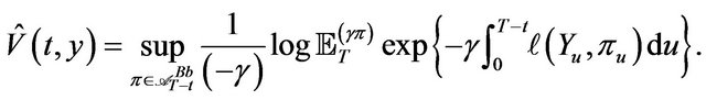
where denotes the expectation with respect to. We now consider, for,

where

The associated HJB equation is written as

(2.13)

By direct calculation, we can see the following.

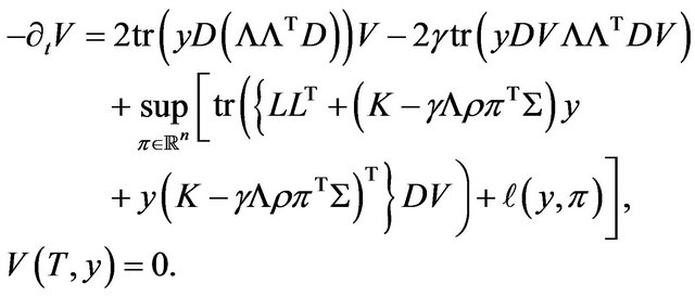
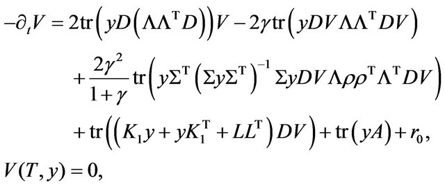
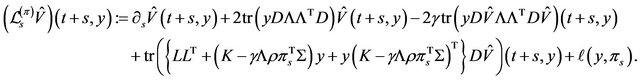
Lemma 2.1 1) If and, then HJB Equation (2.13) is rewritten as

(2.14)

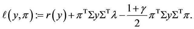
where we define

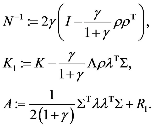(2.15)

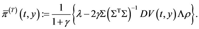
The maximizer for (2.13) is given by

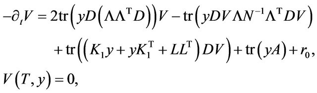
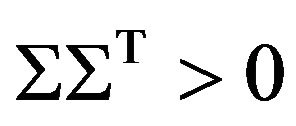2) If and, then HJB equation (2.13) is rewritten as

(2.16)

where and are given by (2.15). The maximizer for (2.13) is given by

3. Results

With the help of Lemma 2.1, it is straightforward to see the following.

Proposition 3.1 (Solution to the HJB equation) 1) If, then

(3.1)

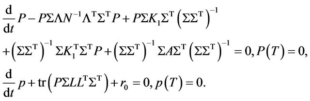
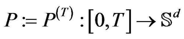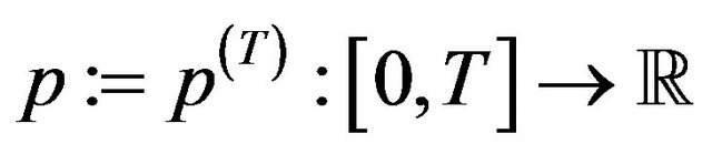solves (2.13), or equivalently (2.14). Here, and solve the following system of ordinary differential equations:

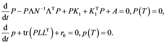(3.2)

2) If, then

(3.3)

solves (2.13), or equivalently (2.16). Here, and solve the following system of ordinary differential equations:

(3.4)

Using this proposition, we obtain the following.

Theorem 3.1 (Verification and optimal strategy)

Define the filtration by

. Let

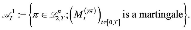
(3.5)

and consider (1.3) with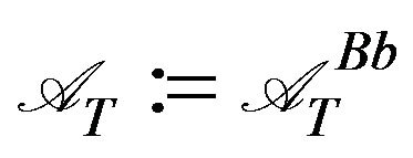. Then, the following assertions hold.

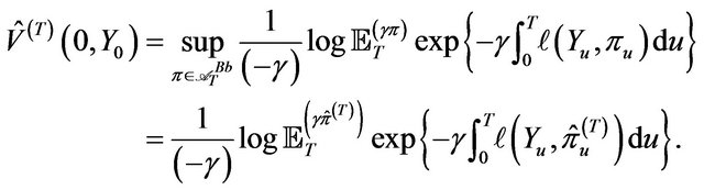
1) If, then, defined by

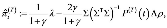(3.6)

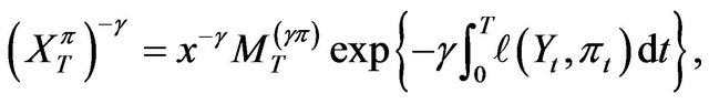
is optimal for (1.3). It holds that

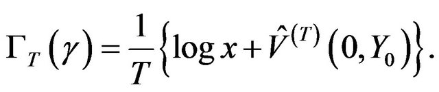(3.7)

2) If, then, defined by

(3.8)

is optimal for (1.3). The relation (3.7) holds.

The proof of the above theorem is given in Subsection 4.2 after preparing lemmas in Subsection 4.1.

4. Proofs

4.1. Lemmas for Exponential Martingale

We prepare the following two lemmas.

Lemma 4.1 Let be -progressively measurable so that

almost surely for all.

Define

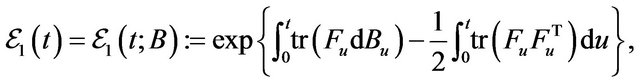
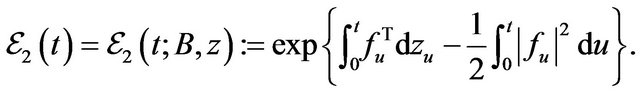
Then, is an -martingale if and only if is an -martingale.

Proof. Denote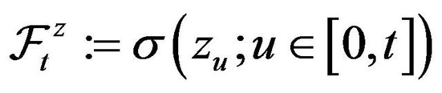. For , we have

Lemma 4.2 Let satisfy the following: for each, is -measurable, and

with some bounded, where we write for. Then, the process, defined by

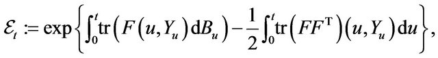
is a martingale.

Proof. The lemma follows from Lemma 4.1.5 of [24], an extension of Lemma 4.1.1 of [25]. Below, we reproduce the proof for self-containedness. Note that it suffices to show

(4.1)

Recall that is progressively measurable. The proof of (4.1) consists of several steps.

First, writing, we recall that

(4.2)

where is defined by (2.8). From this, we can check that

for each with some constant. Also, we can check that

(4.3)

This follows from the relation

(4.4)

where is arbitrary and the constant is independent of. Indeed, in (4.4), letting and using Fatou’s lemma, (4.3) is deduced. To see (4.4), use (2.1) and Itô’s formula to deduce

where we use notation (2.8) and (2.9). From these, we see, from Itô’s formula,

where

is the local-martingale part and is the bounded-variation part, which satisfies

with some constant, independent of. We can check that; hence, is a square-integrable martingale. Further, using (4.2) and recalling that for conformable matrices and, we can check that

with some positive constant, independent of. So, taking the expectation, we deduce that

and that (4.4) follows from Gronwall’s inequality.

Next, use Itô’s formula for the following computation:

(4.5)

Here, we see that

with some constant; hence, the first term of the righthand side of (4.5) is a square-intergrable martingale. Also, we can deduce that

where is a positive constant, independent of. Taking the expectation, we see

Letting and using the dominated convergence theorem, we obtain (4.1).

4.2. Proof of Theorem 3.1

Let be given by (3.1). Fix and take. Using these, define

(4.6)

where we use (2.10), (2.11), and the process given by (2.1), and we set. Using Itô’s formula, we see that

(4.7)

where we define the process by

(see below)

Combining (4.6)-(4.8), we have, for,

Here, note that is a martingale for any by using Lemma 4.1 and 4.2 and that almost everywhere on

since solves HJB-equation

(2.13). So we deduce that is a submartingale for each. Taking the expectation, we see that

Thus, we see that

(4.9)

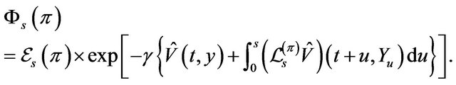
for any. Furthermore, if we define 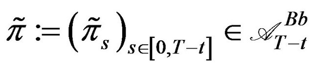by

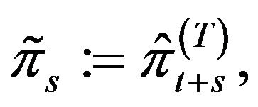
then, we deduce that 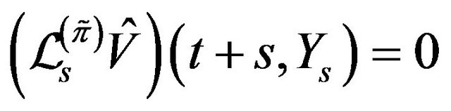almost everywhere on, from which we see that

is a martingale. Therefore, taking the expectation, we see that

that is,

(4.10)

Combining (4.9) and (4.10), we deduce that

(4.11)

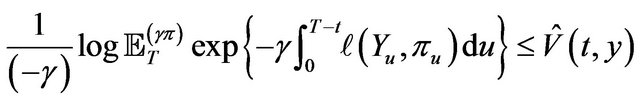
Thus, letting in (4.11), we have that

(4.8)and write

(3.7) follows from relation (2.12).

REFERENCES

- T. R. Bielecki and S. R. Pliska, “Risk Sensitive Dynamic Asset Management,” Applied Mathematics and Optimization, Vol. 39, No. 3, 1999, pp. 337-360. doi:10.1007/s002459900110
- T. R. Bielecki and S. R. Pliska, “Risk Sensitive Intertemporal CAPM, with Application to Fixed-Income Management,” IEEE Transactions on Automat. Control, Vol. 49, No. 3, 2004, pp. 420-432. doi:10.1109/TAC.2004.824470
- M. H. A. Davis and S. Lleo, “Risk-Sensitive Benchmarked Asset Management,” Quantitative Finance, Vol. 8, No. 4, 2008, pp. 415-426.
- W. H. Fleming and S. J. Sheu, “Risk-Sensitive Control and an Optimal Investment Model,” Mathematical Finance, Vol. 10, No. 2, 2000, pp. 197-213. doi:10.1111/1467-9965.00089
- W. H. Fleming and S. J. Sheu, “Risk-Sensitive Control and an Optimal Investment Model. II,” Annals of Applied Probability, Vol. 12, No. 2, 2002, pp. 730-767. doi:10.1214/aoap/1026915623
- H. Hata, H. Nagai and S. J. Sheu, “Asymptotics of the Probability Minimizing a ‘Down-Side’ Risk,” Annals of Applied Probability, Vol. 20, No. 1, 2010, pp. 52-89. doi:10.1214/09-AAP618
- K. Kuroda and H. Nagai, “Risk Sensitive Portfolio Optimization on Infinite Time Horizon,” Stochastics and Stochastics Reports, Vol. 73, No. 3-4, 2002, pp. 309-331.
- M. F. Bru, “Wishart Processes,” Journal of Theoretical Probability, Vol. 4, No. 4, 1991, pp. 725-751. doi:10.1007/BF01259552
- C. Cuchiero, D. Filipovic, E. Mayerhofer and J. Teichmann, “Affine Processes on Positive Semidefinite Matrices,” Annals of Applied Probability, Vol. 21, No. 2, 2011, pp. 397-463. doi:10.1214/10-AAP710
- E. Mayerhofer, O. Pfaffel and R. Stelzer, “On Strong Solutions for Positive Definite Jump Diffusions,” Stochastic Processes and Their Applications, Vol. 121, No. 9, 2011, pp. 2072-2086. doi:10.1016/j.spa.2011.05.006
- A. Benabid, H. Bensusan and N. El Karoui, “Wishart Stochastic Volatility: Asymptotic Smile and Numerical Framework,” Preprint, 2010.
- J. Da Fonseca, M. Grasselli and C. Tebaldi, “Option Pricing When Correlations Are Stochastic: An Analytical Framework,” Review of Derivatives Research, Vol. 10, No. 2, 2007, pp. 151-180. doi:10.1016/j.spa.2011.05.006
- J. Da Fonseca, M. Grasselli and C. Tebaldi, “A Multifactor Volatility Heston Model,” Quantitative Finance, Vol. 8, No. 6, 2008, pp. 591-604. doi:10.1080/14697680701668418
- C. Gouriéroux, “Continuous Time Wishart Process for Stochastic Risk,” Econometric Reviews, Vol. 25, No. 2, 2006, pp. 177-217.
- C. Gouriéroux, J. Jasiak and R. Sufana, “The Wishart Autoregressive Process of Multivariate Stochastic Volatility,” Journal of Econometrics, Vol. 150, No. 2, 2009, pp. 167-181. doi:10.1016/j.jeconom.2008.12.016
- M. Grasselli and C. Tebaldi, “Solvable Affine Term Structure Models,” Mathematical Finance, Vol. 18, No. 1, 2008, pp. 135-153. doi:10.1111/j.1467-9965.2007.00325.x
- A. Buraschi, A. Cieslak and F. Trojani, “Correlation Risk and the Term Structure of Interest Rates,” Working Paper, University of St. Gallen, 2008.
- A. Buraschi, P. Porchia and F. Trojani, “Correlation Risk and Optimal Portfolio Choice,” Journal of Finance, Vol. 65, No. 1, 2010, pp. 393-420. doi:10.1111/j.1540-6261.2009.01533.x
- C. Chiarella, C.-Y. Hsiao and T.-D. Tô, “Risk Premia and Wishart Term Structure Models,” Preprint, 2010.
- C. Gouriéroux and R. Sufana, “Wishart Quadratic Term Structure Models,” Working Paper, CREF, 03-10, HEC, Montreal, 2003.
- D. Duffie, D. Filipovic and W. Schachermayer, “Affine Processes and Applications in Finance,” Annals of Applied Probability, Vol. 13, No. 3, 2003, pp. 984-1053. doi:10.1214/aoap/1060202833
- D. Filipovic and E. Mayerhofer, “Affine Diffusion Processes: Theory and Applications,” Radon Series on Computational and Applied Mathematics, Vol. 8, 2009, pp. 125-164. doi:10.1515/9783110213140.125
- H. Hata, “Down-Side Risk Probability Minimization Problem with Cox-Ingersoll-Ross’s Interest Rates,” AsiaPacific Financial Markets, Vol. 18, No. 1, 2011, pp. 69- 87. doi:10.1007/s10690-010-9121-5
- Y. Watanabe, “Asymptotic Analyses for Certain Stochastic Control Problems under Partial Information and the Related Filtering Equation,” Thesis, Graduate School of Engineering Science, Osaka University, 2011.
- A. Bensoussan, “Stochastic Control of Partially Observable Systems,” Cambridge University Press, Cambridge, 1992. doi:10.1017/CBO9780511526503