Received 27 November 2015; accepted 23 April 2016; published 26 April 2016

ABSTRACT

In this paper, the Box-Jenkins modelling procedure is used to determine an ARIMA model and go further to forecasting. We consider data of Malaria cases from Ministry of Health (Kabwe District)- Zambia for the period, 2009 to 2013 for age 1 to under 5 years. The model-building process involves three steps: tentative identification of a model from the ARIMA class, estimation of parameters in the identified model, and diagnostic checks. Results show that an appropriate model is simply an ARIMA (1, 0, 0) due to the fact that, the ACF has an exponential decay and the PACF has a spike at lag 1 which is an indication of the said model. The forecasted Malaria cases for January and February, 2014 are 220 and 265, respectively.

Keywords:

Box-Jenkins Modeling Procedure, ARIMA Model, Exponential Decay, Spike

1. Introduction

Malaria remains one of the most causes of human morbidity and mortality with a high rate in Africa and Asia. Reference [1] states that, “the vast majority of cases (81%) were in the African region followed by South-East Asia (13%) and Eastern Mediterranean Region (6%)”. There are indications that malaria represents over 10% of Africa’s overall disease burden. Malaria is mostly common in Africa, where it has remained a serious problem accelerating poverty and hindering economic development. Malaria can result in decreased gross domestic product by as much as 1.3% in countries with high disease rates [2] . In this paper, we discuss the Box-Jenkins modeling procedure to determine an ARIMA model and forecast.

The Box-Jenkins approach to forecasting was first described by statisticians George Box and Gwilym Jenkins and was developed as a direct result of their experience with forecast problems in the business, economic, and control engineering applications [3] . Fitting a time series model using the Box-Jenkins modeling procedure allows us to determine an ARIMA (p, d, q) model which is simple and provides a sufficiently accurate description of the behavior of the data. To build a reasonable ARIMA model, as a rule of thumb, Box-Jenkins requires at least 40 or 50 equally-spaced periods of data. The data must also be edited to deal with extreme or missing values or other distortions through the use of functions as log or inverse to achieve stabilization. We need a minimum of n = 50 observations and a number of ACF and PACF to be calculated should be about n/4. The reason why we calculate the ACF and PACF is to use them in identifying the orders of p and q by matching the patterns with the theoretical patterns of known models. A known shortcoming of Box-Jenkins forecasts is that they are based strictly upon univariate analysis, and this limits its use for exploring relationships to time and number of events [4] . Box-Jenkins forecasting is of greatest use when the underlying factors causing demand for products, services, revenue, and, in this case, disease burden is believed to behave in the future in much the same manner as it did in the past [5] .

The application significance of this study is that by developing forecasting models for predicting the expected number of malaria cases in advance, timely prevention and control measures can be effectively planned like eliminating vector breeding places, spraying insecticides, and creating public awareness.

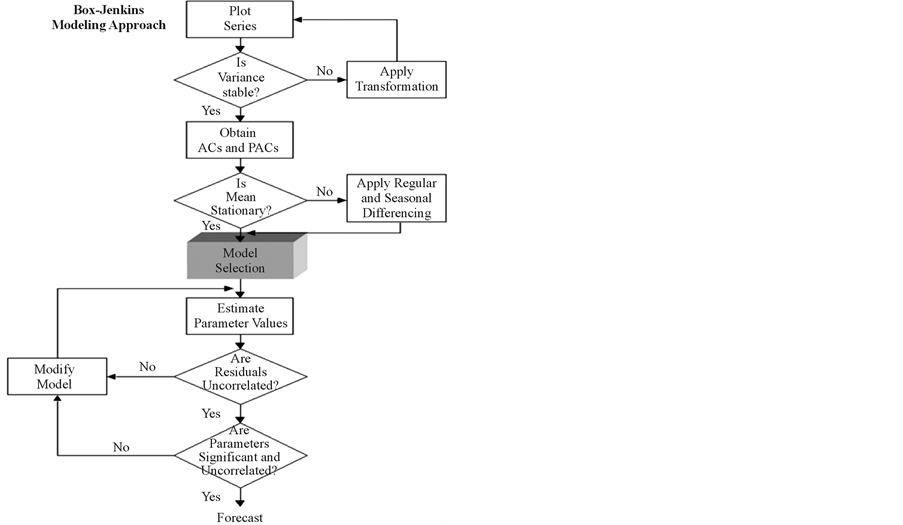
The model-building process involves three steps.

1) Tentative identification of a model from the ARIMA class.

2) Estimation of parameters in the identified model.

3) Diagnostic checks.

Tentative identification of model―at this stage we use two graphical devices which are the estimated autocorrelation function (ACF) and an estimated partial autocorrelation function (PACF) as guides to choosing one or more Autoregressive Integrated Moving Average (ARIMA) models that are appropriate.

Estimation of parameters in the identified model―at this stage we get precise estimate of the coefficients of the model chosen at the identification stage.

Diagnostic checks―used to help determine if an estimated model is statistically adequate.

If the tentatively identified model passes the diagnostic tests, the model is ready to be used for forecasting. If it does not, the diagnostic tests should indicate how the model ought to be modified, and a new cycle of identification, estimation and diagnosis is performed. With a stationary series in place, a basic model can now be identified. Three basic models exist, AR (autoregressive), MA (moving average) and a combined ARMA. When regular differencing is applied together with AR and MA, they are referred to as ARIMA, with the “I” indicating “integrated”. The general ARIMA (p, d, q) model is defined as

(1)

where, , and the series e_t is a Gaussian white noise process.

The paper is organized as follows: In Section 2, we give brief survey on previous works (literature review). In Section 3 we display the data set used in this paper. Section 4 we discuss the modelling approach together with the model used in this paper. The forecasting results are presented in Section 5 and the conclusion is presented in Section 6.

2. Literature Review

A brief survey on previous work provides the context of this paper.

Reference [6] observed that malaria transmission in most areas was highly variable from season-to-season and year-to-year. In their study, different methods were compared with forecast of malaria incidence from historical morbidity patterns in areas with unstable transmission to access their potential use in epidemic early warning. It was noted that the potential use of time series techniques especially the ARIMA method in epidemiological studies, disease surveillance and outbreak forecast, has been explored in some studies. The method of using seasonal adjustment were found to produce relatively better forecast of malaria incidences compared with the ARIMA method and there reason was that the method of seasonal adjustments takes account of deviations from seasonal averages of last three observations which gave the best forecast compared with other methods. The method was also defended in terms of its capability to accommodate both seasonality and recent changes or trends at the same time while other studies have also indicated that the statistically advanced ARIMA models may produce very good fit to the data but in post-sample forecast, they would not be robust enough to handle a possible change in behavior of series. The results of the study indicate the need for balancing short historical and long enough series to minimize the random error and it was observed in the results of the analysis which showed that simple methods such as seasonal adjustments perform as well as or even better than the more advanced ARIMA method. Reference [7] in their paper examined the modeling and forecasting malaria mortality rate using SARIMA Models. They argued that among the most effective approaches for analyzing time series data is the method propounded by Box and Jenkins, the Autoregressive Integrated Moving Average (ARIMA). In this paper, Box-Jenkins methodology to build ARIMA model for malaria mortality rate for the period January 1996 to December 2013 with a total of 216 data points was employed. The model obtained in this paper was then used to forecast monthly malaria mortality rate for the upcoming year 2014. They stated that, the forecasted results would help Government and medical professionals to see how to maintain steady decrease of malaria mortality in other to combat the predicted rise in mortality rate envisaged in some months. Reference [8] conducted a study titled “Increasing Burden of Childhood Severe Malaria in a Nigerian Tertiary Hospital: Implication for control, between January 2000 and December 2005”. Using logistic Regression, the result showed that severe Malaria constituted an important cause of hospital admission among Nigerian children especially those aged below 5 years. The result also revealed that there was significant increase in the proportion of cases of severe malaria from 2000 to 2005. Reference [9] states that malaria still remains a public health problem in developing countries and changing environmental and climatic factors pose the biggest challenge in fighting against the scourge of malaria. Their study was designed to forecast malaria cases using climatic factors as predictors in Delhi, India. The total number of monthly cases of malaria slide positives occurring from January 2006 to December 2013 was taken from the register maintained at the malaria clinic at Rural Health Training Centre (RHTC) Delhi. Climatic data of monthly mean rainfall, relative humidity, and mean maximum temperature were taken from Regional Meteorological Centre, Delhi. SPSS 21 was used for analyzing the time series data. Results show that the Autoregressive integrated moving average, ARIMA (0, 1, 1) (0, 1, 0) 12, was the best fit model and it could explain 72.5% variability in the time series data. Rainfall (P value = 0.004) and relative humidity (P value = 0.001) were found to be significant predictors for malaria transmission in the study area. Seasonal adjusted factor (SAF) for malaria cases showed peak during the months of August and September. Finally, they concluded that ARIMA model of time series analysis is a simple and reliable tool for producing reliable forecasts for malaria in Delhi, India. Reference [10] in their paper modelled the evolution of monthly unemployment rate from January, 1998 to December, 2007 using the Box-Jenkins methodology. Results in their paper showed that the most adequate model for the unemployment rate was an ARIMA (2, 1, 2). They went further to forecasts the values of unemployment rate for January and February, 2008 and found out that the unemployment rate for January, 2008 was 4.06%.

3. A Numerical Example

The data from Table 1 consists of 60 monthly Malaria cases from January 2009 to December 2013 for age 1 to under 5 years. 2014 data set was not ready at the time of collection. This study assumes that the reporting and registering of monthly malaria cases remain the same throughout the study period. Since the study was done by collecting data from a single centre, it is difficult to generalize the results in the actual population.

4. Model-Building Process

The first step in this time series analysis is to plot the observations against time. Graphs from these observations are called time plot and they show up important features of the series such as trend, seasonality, outliers and discontinuities. The input data must be adjusted to form a stationary series, one whose values vary more or less uniformly about a fixed level over time. Trends can be adjusted by “regular differencing”, a process of computing the difference between every two successive values, computing a differenced series which has overall trend behavior removed. If a single differencing does not achieve stationarity, it may be repeated although rare to have more than two regular differencing’s. Where irregularities in the differenced series continue to be displayed, log or inverse functions can be specified to stabilize the series such that the remaining residual plot displays values approaching zero and without any pattern. This is the error term, equivalent to pure, white noise [11] .

A visual inspection of the time series plot in Figure 1 suggests a stationary process with constant mean and variance.

4.1. Model Selection

Two graphical devices which are the autocorrelation function (ACF) and partial autocorrelation function (PACF) are used as guides to choosing one or more Autoregressive Integrated Moving Average (ARIMA) models that are appropriate.

Figure 2 describe the features of the data that is the autocorrelation plot and the partial autocorrelation plot. The ACF and PACF show that the ACF decays exponentially and the PACF has a single spike at lag 1 indicating that the series is generated by an ARIMA (1, 0, 0) process,

(2)

Source: Ministry of Health-Kabwe District Community Medical Office (KDCMO).

4.2. Parameter Estimation

Equation (2) can now be used to estimate the parameter by least squares estimation. Reference [12] argue that because the method of moments is unsatisfactory for many models, we will consider the method of least squares estimation for our model. Given that our identified model is.

We view this as a regression model with predictor variable X_t then apply the Least Squares estimation proceeds by minimizing the sum of the differences. The estimators are and can be obtained as follows:

(3)

(4)

Calculations in Excel show that: and. Hence, the model is

(5)

4.3. Diagnostic Checks

Verification of goodness of fit of any model should include a test as to whether the residuals form a white noise process. A portfolio of tests for goodness of fit of our model has been done in this paper.

The histogram shows that the average of residuals is approximately 0. The QQ plots are an effective tool for assessing normality. The QQ plot of residual observations in Figure 3 suggests that the points follow the straight line (45 degree line) closely implying that the residuals are normally distributed.

The autocorrelation plot show (see Figure 4) that only one value is outside the confidence limit which would not be regarded as significant on its own, three such values might be considered to be significant. All the terms of the partial autocorrelation plot are interior to the confidence limit suggesting that the residuals are a white noise.

Our other diagnostic check is to inspect a scatter plot of the residuals over time in Figure 5. The model is adequate, since the residual scatter plot show a rectangular scatter around a zero horizontal level with no trends present.

5. Forecasting

Box-Jenkins approach to forecasting stationary time series is relatively simple. The forecast value of given all observations up until n the k-step ahead forecast is denoted by. The one-step ahead and two- step ahead forecasts for an ARIMA (1, 0, 0) are given by:

(6)

and

(7)

The general form of the forecast equation is therefore

(8)

for. We want to forecast with and considering the data in Table 1.

.

6. Discussion

ARIMA (1, 0, 0) model developed in this paper attempts to provide the best possible model for predicting malaria cases per month in the future based on observed malaria cases over the years. The results also indicate that the malaria cases will continue to occur in the near future if appropriate intervention measures are not initiated on time. The potential implication of this study is that by developing forecasting models for predicting the expected number of malaria cases in advance, timely prevention and control measures can be effectively planned like eliminating vector breeding places, spraying insecticides, and creating public awareness. The study also provides a model to foresee and allocate appropriate resources to maintain a steady decrease and combat malaria. The ARIMA model used in this paper can also be applied to other diseases like Ebola. These results can also be used to sensitize travelers about malaria risk to take necessary precautionary measures.

7. Conclusion

In this paper, the Box-Jenkins modelling procedure is discussed to determine an ARIMA model and go further to forecasting. We considered data of Malaria cases from Ministry of Health (Kabwe District)-Zambia for the period, 2009 to 2013 for age 1 to under 5 years. Results show that an appropriate model is simply an ARIMA (1, 0, 0) due to the fact that, the ACF decays exponentially and the PACF has a spike at lag 1 which is an indication of the said model. The forecasted Malaria cases for January and February, 2014 are 220 and 265, respectively. Finally, the study can be done on a wider area of Zambia and further research can be done to evaluate the effectiveness of integrating the forecasting model into the existing disease control program in terms of its impact in reducing the disease occurrence. These will be studied elsewhere.

Acknowledgements

The authors are thankful to the Ministry of Health for providing the data. Department of Mathematics and Statistics, Mulungushi University for using their resources and to all the people who helped in making comments on this paper.

Cite this paper

Stanley Jere,Edwin Moyo, (2016) Modelling Epidemiological Data Using Box-Jenkins Procedure. Open Journal of Statistics,06,295-302. doi: 10.4236/ojs.2016.62025

References

NOTES

^*Corresponding author.

References

- 1. Abebe, A., Dagnachew, M., Mikrie, M., Meaza, A. and Melkamu, G. (2012) Ten Year Trend Analysis of Malaria Prevalence in Kola Diba, North Gondar, Northwest Ethiopia. Parasites and Vectors, 5, 173.
http://dx.doi.org/10.1186/1756-3305-5-173 - 2. World Health Organization (2011) World Malaria Report. Geneva, Switzerland.
www.who.int/malaria/world_malaria_report_2011 - 3. Box, G.E. and Jenkins, G.M. (1994) Time Series Analysis: Forecasting and Control. Prentice Hall, Englewood Cliffs.
- 4. Pankratz, A. (1983) Forecasting with Univariate Box-Jenkins Models. Wiley & Sons, Inc., New York.
http://dx.doi.org/10.1002/9780470316566 - 5. Levenback, H. and Cleary, J.P. (2006) Forecasting Practice and Process for Demand Management. Thomson Brooks/ Cole, Belmont.
- 6. Tarekegn, A.A., Sake, J.D., Gerard, B., Awash, T., Asnakew, K., Dereje, O., Gerrit, J. and Habbema, J.D.F. (2002) Forecasting Malaria Incidence from Historical Morbidity Patterns in Epidemic-Prone Areas of Ethiopia: A Simple Seasonal Adjustment Method Performs Best. Tropical Medicine and International Health, 7, 851-857.
http://dx.doi.org/10.1046/j.1365-3156.2002.00924.x - 7. Ekezie, D.D., Opara, J. and Okenwe, I. (2014) Modelling and Forecasting Malaria Mortality Rate Using SARIMA Models (A Case Study of Aboh Mbaise General Hospital, Imo State Nigeria). Science Journal of Applied Mathematics and Statistics, 2, 31-41.
http://dx.doi.org/10.11648/j.sjams.20140201.15 - 8. Adebola, P.A. and Okereke, R.W. (2007) Increasing Burden of Childwood Severe Malaria in a Nigeria Tertiary Hospital from 2000 to 2005. An Unpublished Research Work.
- 9. Varun, K., Abha, M., Sanjeet, P., Geeta, Y., Richa, T., Deepak, R. and Saudan, S. (2014) Forecasting Malaria Cases Using Climatic Factors in Delhi, India: A Time Series Analysis. Hindawi Publishing Corporation Malaria Research and Treatment, 2014, Article ID: 482851.
- 10. Dobre, I. and Alexandru, A. (2008) Modelling Unemployment Rate Using Box-Jenkins Procedure. Journal of Applied Quantitative Methods, 3.
- 11. Wei, W. (1990) A Time Series Analysis: Univariate and Multivariate Methods. Addison-Wesley Publishing Company, Inc., New York.
- 12. Cryer, J.D. and Chan, K.S. (2008) Time Series Analysis with Application in R. Springer, New York.
http://dx.doi.org/10.1007/978-0-387-75959-3