Open Journal of Statistics
Vol.4 No.4(2014), Article
ID:47087,22
pages
DOI:10.4236/ojs.2014.44030
Factor Vector Autoregressive Estimation of Heteroskedastic Persistent and Non Persistent Processes Subject to Structural Breaks
Claudio Morana1,2
1Department of Economics, Management and Statistics, University of Milan, Milan, Italy
2Center for Research on Pensions and Welfare Policies, Collegio Carlo Alberto, Moncalieri, Italy
Email: claudio.morana@unimib.it
Copyright © 2014 by author and Scientific Research Publishing Inc.
This work is licensed under the Creative Commons Attribution International License (CC BY).
http://creativecommons.org/licenses/by/4.0/


Received 22 March 2014; revised 18 April 2014; accepted 6 May 2014
ABSTRACT
In the paper, a general framework for large scale modeling of macroeconomic and financial time series is introduced. The proposed approach is characterized by simplicity of implementation, performing well independently of persistence and heteroskedasticity properties, accounting for common deterministic and stochastic factors. Monte Carlo results strongly support the proposed methodology, validating its use also for relatively small cross-sectional and temporal samples.
Keywords:Long and Short Memory, Structural Breaks, Common Factors, Principal Components Analysis, Fractionally Integrated Heteroskedastic Factor Vector Autoregressive Model

1. Introduction
In the paper, a general strategy for large-scale modeling of macroeconomic and financial data, set within the factor vector autoregressive model (F-VAR) framework, is proposed.1
Following the lead of dynamic factor model analysis proposed in [2] , it is assumed that a small number of structural shocks are responsible for the observed comovement in economic data; it is, however, also assumed that commonalities across series are described by deterministic factors, i.e., common break processes. Comovement across series is then accounted by both deterministic and stochastic factors; moreover, common factors are allowed in both mean and variance, covering the I(0) and I(1) persistence cases, as well as the intermediate case of long memory, i.e., I(d), . As the common factors are unobserved, accurate estimation may fail in the framework of small scale vector autoregressive (VAR) models, but succeed when cross-sectional information is employed to disentangle common and idiosyncratic features.
The proposed fractionally integrated heteroskedastic factor vector autoregressive model (FI-HF-VAR) bridges the F-VAR and (the most recent) G-VAR literature, as, similarly to [3] , a weakly stationary cyclical representation is employed; yet, similarly to [4] , principal components analysis (PCA) is employed for the estimation of the latent factors. Consistent and asymptotically normal estimation is performed by means of QML, also implemented through an iterative multi-step estimation procedure. Monte Carlo results strongly support the proposed methodology.
Overall, the FI-HF-VAR model can be understood as a unified framework for large-scale econometric modeling, allowing for accurate investigation of cross-sectional and time series features, independent of persistence and heteroskedasticity properties of the data, from comovement to impulse responses, forecast error variance and historical decomposition analysis.
After this introduction, the paper is organized as follows. In Section 2, the econometric model is presented; in Section 3, estimation is discussed, while Monte Carlo analysis is performed in Section 4; finally, conclusions are drawn in Section 5.
2. The FI-HF-VAR Model
Consider the following fractionally integrated heteroskedastic factor vector autoregressive (FI-HF-VAR) model
 (1)
(1)

 (2)
(2)

where  is a
is a  vector of real valued integrated I(d) (
 ) and heteroskedastic processes subject to structural breaks,
  in deviation from the unobserved common deterministic (
 ) and stochastic (ft)
factors;  is a finite order matrix of polynomials in the lag operator with all the roots outside the unit circle,
  ,
,  , is a square matrix of coefficients of order N;
  is a
is a
 vector of zero mean idiosyncratic i.i.d. shocks, with contemporaneous covariance matrix
 , assumed to be coherent with the condition of weak cross-sectional correlation of the idiosyncratic components (Assumption E) stated in [5] p. 143. The model in (1) actually admits the same static representation of [5] , as it can be rewritten as
 .
.
2.1. The Common Break Process Component
The vector of common break processes  is
is , with
 , and
, and  matrix of loadings
 ; the latter are assumed to be orthogonal to the common stochastic factors
 , and of unknown form, measuring recurrent or non recurrent changes in mean, with smooth or abrupt transition across regimes; the generic element in μt is μi,t≡zμ,i(t), where
  is a function of the time index t,
 .
.
The idiosyncratic break process  can take different forms. For instance, [6] use a discontinuous function,
 (3)
(3)
where  is the indicator function, such that
  if
if  and is 0 otherwise; in [6] the break points
are determined through testing; a Markov switching mechanism, as in [7] , could however also be employed to this purpose.
Differently, [8] [9] and [10] model the break process as a continuous and bounded function of time, by means of a Fourier expansion, i.e.,
 (4)
(4)
Similarly [11] , using a logistic specification
 (5)
(5)
where the logistic function is ,
,  ,
,  and
and
 are parameters,
  , and
, and  is the estimated standard deviation of
 . In particular, as
 ,
,
 becomes the indicator function, yielding therefore a generalization of the specification in [6] .
Also similarly [12] and [13] , using a spline function
 , (6)
, (6)
where  is a spline function of order p,
  are unknown regression coefficients and the functions
  are spline basis functions defined as
 ,
,  ,
, ,
,  , and
, and
 , with
 .
.
A semiparametric approach has also been suggested by [14] , using a kernel function, i.e.,
 , (7)
, (7)
where b is the bandwidth and  is the kernel function, specified as
  for
for  and
and
 for
for ;
;  and the coefficient
  are such that
 .
.
Finally, a random level shift model has been proposed by [15] -[18] ; for instance, [18] define the break process as
 (8)
(8)
where  and
and  for
for .
.
In the case , there are no common break processes, i.e., each series is characterized by its own idiosyncratic break process and the
  factor loading matrix
  is square, diagonal and of full rank; when
 , there exist M common break processes and the factor loading matrix is of reduced rank (M). Hence, in the latter case the series
  are cotrending, according to [19] , nonlinear cotrending, according to [20] , or cobreaking, according to [21] and [22] . The representation in (1) emphasizes however the driving role of the common break processes, rather than the break-free linear combinations (cobreaking/cotrending relationships) relating the series
 .
.
2.2. The Common Break-Free Component
The vector of (zero-mean) integrated heteroskedastic common factors  is
is , with
 , and
, and 
matrix of loadings . The order of integration is
  in mean, and
  in variance,
  ,
,  ,
,
 .
.
The polynomial matrix  is of finite order, with all the roots outside the unit circle;
 ,
,  , is a square matrix of coefficients of order
 ;
;  is a
is a  vector of common zero mean i.i.d. shocks, with identity covariance matrix
 ,
,  all
all , respectively.
The matrix  is a square diagonal matrix in the lag operator of order
 , specified according to the integration order (in mean) of the common stochastic factors, i.e.,
  for the case of
  integration (
 );
); for the
  or no integration (short memory) case (
 );
);
 for the case of fractional integration (
 , long memory)
( ), where
  is the fractional differencing operator; the latter admits a binomial expansionwhich can be compactly written in terms of the Hypergeometric function, i.e.,
 , where
  is the Gamma function.
In the case  there are no common stochastic processes, i.e., each series is characterized by its own idiosyncratic persistent stochastic component, and the
  factor loading matrix
  is square, diagonal and of full rank; when
 , then there exist R common stochastic processes and the factor loading matrix is of reduced rank (R). Hence, in the latter case the series
  show common stochastic features, according to [23] . The concept of common feature is broad, encompassing the notion of cointegration ([24] ), holding for the
  case. The representation in (1) emphasizes however the driving role of the common stochastic factors rather than the feature-free linear combinations (cofeature relationships) relating the series
 .
.
2.3. The Conditional Variance Process
The  conditional variance-covariance matrix for the unconditionally and conditionally orthogonal common factors
  is
is , where
  is the information set available at time period
 . Consistent with the constant conditional correlation model of [25] , the ith generic element along the main diagonal of
  is
is
 (9)
(9)
where  for the case of fractional integration (long memory) in variance
( );
); for the case of
  integration in variance (
 );
);
 for the
  or no integration (short memory) in variance case (
 ). In all cases
 ,
,  ,
,  ,
,
 and all the roots of the
  and
and  polynomials are outside the unit circle.
The conditional variance process ,
,  , is therefore of the
type [26] , with , or the
  type, for the fractionally integrated and integrated case, respectively; of the
  type for the non integrated case. The model is however not standard as the intercept component
  is time-varying, allowing for structural breaks in variance; similarly to the mean part of the model, structural breaks in variance are assumed to be of unknown form, measuring recurrent or non recurrent regimes, with smooth or abrupt transition; then,
  , where
  is a continuos or discontinuous bounded function of the time index
 ,
,  , which can be parameterized as in (3), (4), (5), (6), (7), or (8).
The following ARCH (∞) representation can be obtained from each of the three above models
 (10)
(10)
where  and
and .
.
The term  then bears the interpretation of break in variance process, or time-varying unconditional variance process (no integration case), or long-term conditional variance level (unit root and fractional integration cases).
To guarantee the non negativity of the conditional variance process at eachpoint in time all the coefficients in the  representation must be non-negative, i.e.,
  for all
  and
and  for any
 . Sufficient conditions, for various parameterization, can be found in [26] and [27] .
2.4. The Reduced Fractional VAR form
By substituting (2) into (1) and rearranging, the vector autoregressive representation for the factors  and the gap series
  can be written as
 (11)
(11)

where  and
and  is differently defined according to persistence properties of the data. In particular, for the case of fractional integration (long memory)
 , by means of the binomial expansion, it follows
 ,
,  , where
 ,
,  , is a square matrix of coefficients of dimension
 , and
, and ; since the infinite order representation cannot be handled in estimation, a truncation to a suitable large lag for the polynomial matrix
  is required.2 Hence,
 . For the case of no integration (short memory) (
 ), recalling that
  , and therefore
 , then
 ; for the case of integration (
 ), it should be firstly recalled that
 , with
 ; the latter may be rewritten in the equivalent polynomial matrix form
 , where
 ,
,  , is a square matrix of coefficients of dimension
 , and
, and ,
,
 ; then,
 .
.
Reduced Form and Structural Vector Moving Average Representation of the FI-HF-VAR Model
In the presence of unconditional heteroskedasticity, the computation of the impulse response functions and the forecast error variance decomposition (FEVD) should be made dependent on the estimated unconditional variance for each regime. In the case of (continuously) time-varying unconditional variance, policy analysis may then be computed at each point in time. For some of the conditional variance models considered in the paper, i.e., the FIGARCH and IGARCH processes, the population unconditional variance does not actually exist; in the latter cases the  component might bear the interpretation of long term level for the conditional variance; policy analysis is still feasible, yet subject to a different interpretation, FEVD referring, for instance, not to the proportion of forecast error (unconditional) variance accounted by each structural shock, but to the proportion of forecast error (conditional) long term variance accounted by each structural shock. With this caveat in mind, the actual computation of the above quantities is achieved in the same way as in the case of well defined population unconditional variance.
Hence, the computation of the vector moving average (VMA) representation for the FI-HF-VAR model depends on the persistence properties of the data. The following distinctions should then be made.
For the short memory case, i.e., the zero integration order case , the VMA representation for the factors
  and gap series
  can be written as
 , (12)
where ,
,  and
and .
.
For the long memory case ( ) and the case of
  non stationarity (
 ), the VMA representation should be computed for the differenced process, yielding
 , (13)
where ,
,  and
and . Impulse responses can then be computed as
  for
for  and
and  and
and  for
for ,
, 
The identification of the structural shocks in the FI-HF-VAR model can be implemented in two steps. Firstly, denoting by  the vector of the
  structural common factor shocks, the relation between reduced and structural form common shocks can be written as
 , where
  is square and invertible. Therefore, the identification of the structural common factor shocks amounts to the estimation of the elements of the
  matrix. It is assumed that
 , and hence
 . As the number of free parameters in
  is
is
 , at most
  parameters in
  can be uniquely identified through the
system of nonlinear equations in the unknown parameters of . Additional
  restrictions need then to be imposed for exact identification of
 , by constraining the contemporaneous or long-run responses to structural shocks; for instance, recursive (Choleski) or non recursive structures can be imposed on the VAR model for the common factors through exclusion or linear/non-liner restrictions, as well as sign restrictions, on the contemporaneous impact matrix
 .3
.3
Secondly, by denoting  the vector of
  structural idiosyncratic disturbances, the relation between reduced form and structural form idiosyncratic shocks can be written as
 , where K is square and invertible. Hence, the identification of the structural idiosyncratic shocks amounts to the estimation of the elements of the K matrix. It is assumed that
 , and hence
 . Then, in addition to the
  equations provided by
 ,
,  restrictions need to be imposed for exact identification of
 similarly to what required for the common structural shocks.
Note that preliminary to the estimation of the  matrix,
  should be obtained from the residuals of an OLS regression of
  on
on ; the latter operation would grant orthogonality between common and idiosyncratic residuals.
The structural VMA representation can then be written as
 , (14)
where ,
,  ,
,  , or
, or
 , (15)
where ,
,  ,
,  , according to persistence properties, and
  any
any .
.
3. Estimation
Estimation of the model can be implemented following a multi-step procedure, consisting of persistence analysis,  estimation of the common factors and VAR parameters in (1),
  estimation of the conditional mean model in (2) and the reduced form model in (11),
  estimation of the conditional variance covariance matrix in (2).
3.1. Step 1: Persistence Analysis
Each component ,
,  , in the vector time series
  is firstly decomposed into its purely deterministic (trend/break process;
 ) and purely stochastic (break-free,
 ) parts.
It is then assumed that the data obey the model
 , (16)
where  and
and  are orthogonal,
  , with
  a bounded function of the time index
 , evolving according to discontinuous changes (step function) or showing smooth transitions across regimes.
Depending on the specification of , a joint estimate of the two components can be obtained following [7] [10] [11] [13] [14] [30] , by setting up an augmented fractionally integrated ARIMA model
 , (17)
where  is the integer differencing parameter,
  is the fractional differencing parameter
( ),
), is a stationary polynomial in the lag operator and
  is a white noise disturbance.
Heteroskedastic innovations can also be considered, by specifying , with
 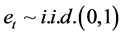 and the conditional variance process
  according to a model of the GARCH family.
Consistent and asymptotically normal estimation by means of , also implemented through iterative algorithms, is discussed in [10] [13] [14] [18] [31] . Extensions of the Markov switching [7] , logistic [11] and random level shift [15] -[18] models to the long memory case have also been contributed by [32] [33] and [34] , respectively.
Alternatively, following [6] , a two-step procedure can be implemented: firstly, structural break tests are carried out and break points estimated; then, dummy variables are constructed according to their dating and the break process is estimated by running an OLS regression of the actual series  on the latter dummies, as in (3); this yields
  computed as the fitted process and the stochastic part as the estimated residual, i.e.,
 ;
;
 and
and  are then orthogonal by construction.4
As neglected structural breaks may lead to processes which appear to show persistence of the long memory or unit root type, as well as spurious breaks may be detected in the data when persistence in the error component is neglected, testing procedures robust to persistence properties are clearly desirable. In this respect, the RSS-based testing framework in [6] yields consistent detection of multiple breaks at unknown dates for  processes, as well as under long range dependence [35] ;5 moreover, under long range dependence, the validity of an estimated break process (obtained, for instance, by means of [6] ) may also be assessed by testing the null hypothesis of long memory in the estimated break-free series (
 ), as antipersistence is expected from the removal of a spurious break process [36] [37] . Structural break tests valid for both
  and
and  series have also recently contributed in the literature.
3.2. Step 2: Estimation of the Conditional Mean Model
 estimation of the reduced form model in (11) is performed by first estimating the latent factors and VAR parameters in (1); then, by estimating the conditional mean process in (2); finally, by substituting (2) into (1) in order to obtain a restricted estimate of the polynomial matrix
 .
.
3.2.1. Estimation of the Common Factors and VAR Parameters
Estimation of the common factors is performed by , writing the (misspecified) approximating model as
 (18)
(18)


with log-likelihood function given by
 . (19)
QML estimation of the latent factors and their loadings then requires the minimization of the objective function
 (20)
(20)
which can be rewritten as
 , (21)
where , as
, as  and
and  are orthogonal vectors, as well as
  and
and .
.
The solution to the minimization problem, subject to the constraints  and
and![]() , is given by firstly minimizing with respect to
, is given by firstly minimizing with respect to  and
and , given
  and
and , yielding


and then concentrating the objective function to obtain
 , (22)
which can be mimized with respect to  and
and . This is equivalent to maximizing
 , (23)
which in turn is equivalent to maximizing
 (24)
(24)
subject to , and
, and
 (25)
(25)
subject to .
.
The solution is then found by setting:
Ÿ  equal to the scaled eigenvectors of
 , i.e., the sample variance covariance matrix of the break processes
 , associated with its
  largest eigenvalues; this yields
 , i.e., the scaled first
principal components of ;
;
Ÿ  equal to the scaled eigenvectors of
 , i.e., the sample variance covariance matrix of the break-free processes
 , corresponding to its
  largest eigenvalues; this yields
 , i.e., the scaled first
principal components of .
.
Note that PCA uniquely estimates the space spanned by the unobserved factors; hence,  and
and  (
(
and ) are not separately identified, as the common factors
  and factor loading matrix
  are uniquely estimated up to a suitable invertible rotation matrix
 , i.e., PCA delivers estimates of
 and
and , and therefore a unique estimate of the common components
  only, which is however all what is required for the computation of the gap vector.
As shown by [38] , exact identification of the common factors can also be implemented, by appropriately constraining the factor loading matrix while performing PCA or after estimation. In particular, three identification structures are discussed, involving a block diagonal factor loading matrix, yield by a statistical restriction imposed in estimation, and two rotation strategies, yielding a lower triangular factor loading matrix in the former case and a two-block partitioned factor loading matrix in the latter case, with identity matrix in the upper block and an unrestricted structure in the lower block.
Moreover, the number of common factors  is unknown and needs to be determined; several criteria are available in the literature, ranging from heuristic or statistical eigenvalue-based approaches [39] [40] to the more recent information criteria [41] and “primitive” shock ([42] ) based procedures.
Finally, in order to enforce orthogonality between the estimated common break processes  and stochastic factors
 , the above procedure may be modified by computing the stochastic component
  as the residuals from the OLS regression of
  on
on ; then PCA is implemented on (the break-free residuals)
  to yield
 .
.
Estimation of the VAR parameters. Conditional on the estimated (rotated) latent factors, the polynomial matrix  and the
  and
and  (rotated) factor loading matrices are obtained by means of OLS estimation of the equation system in (1). This can be obtained by first (OLS) regressing the actual series xt on the estimated common break processes
  and stochastic factors
  to obtain
  and
and ;
;
alternatively,  and
and  can be estimated as yield by PCA, i.e., from the scaled eigenvectors of the matrices
  and
and , respectively; then, the gap vector is computed as
 , as
, as  and
and
 , and
, and  is obtained by means of OLS estimation of the VAR model in (1).
3.2.2. Iterative Estimation of the Common Factors and VAR Parameters
The above estimation strategy may be embedded within an iterative procedure, yielding a (relatively more efficient) estimate of the latent factors and the VAR parameters in the equation system in (1).
The objective function to be minimized is then written as
 (26)
(26)
where .
.
Ÿ Initialization. The iterative estimation procedure requires an initial estimate of the common deterministic  and stochastic
  factors and the
  polynomial matrix, i.e., an initial estimate of the equation system in (1). The latter can be obtained as described in Section 3.2.1.
Ÿ Updating. An updated estimate of the equation system in (1) is obtained as follows.
° First, a new estimate of the  (rotated) common deterministic factors, and their factor loading matrix, is obtained by the application of PCA to the (new) stochastic factor-free series
 , yielding
  and
and .6
.6
° Next, conditional on the new common break processes and their factor loading matrix, the new estimate of the common long memory factors is obtained from the application of PCA to (new) break-free processes
 7 yielding
  and
and .8
.8
° Finally, conditional on the new estimated common break processes and long memory factors, the new estimate of the gap vector  is obtained, and the new estimate
  can be computed by means of OLS estimation of the VAR model in (1).
° The above procedure is iterated until convergence, yielding the final estimates ,
,  and
and . Convergence may be assessed in various ways. For instance, the procedure may be stopped when the change in the value of the objective function is below a given threshold.9
3.2.3. Restricted Estimation of the Reduced Form Model
Once the final estimate of the equation system in (1) is available, the reduced VAR form in (11) is estimated as follows:
1) For the case of fractional integration (long memory) ( ), the fractional differencing parameter is
(consistently) estimated first, for each component of the (rotated) common factors vector , yielding the estimates
 ,
,  , collected in
  matrix.
Considering then the generic element ,
,  consistent and asymptotically normal estimation of the ith fractional differencing parameter can be obtained, for instance, by means of
  estimation of the fractionally integrated ARIMA model in (17); alternatively, consistent and asymptotically normal estimation can be obtained by means of the log-periodogram regression or the Whittle-likelihood function.10
Then, conditionally to the estimated fractionally differencing parameter,  is obtained by means of OLS estimation of the
  model for the fractionally differenced common factors
  in (2); hence,
 , where
  is the diagonal polynomial matrix in the lag operator of order R, containing the
  th order
  truncated binomial expansion of the elements in
 . Then,
 and
and .
.
Alternatively, rather than by means of the two-step Box-Jenkins type of approach detailed above, VARFIMA estimation of the R-variate version of the model in (17) can be performed by means of Conditional-Sum-ofSquares [45] , exact Maximum Likelihood [46] or Indirect [47] estimation, still yielding  consistent and asymptotically normal estimates.11 OLS estimation of a VAR approximation for the VARFIMA model has also been recently proposed in [48] , which would even avoid the estimation of the fractional differencing parameter for the common stochastic factors.
For the case of no integration (short memory) ( ) and integration (
 ), we also have:
2) For the case of no integration (short memory) ( ),
), is obtained by means of OLS estimation of the VAR(u) model for the (rotated) common stochastic factors (
 ) in (2); then
 ;
;
3) For the  case (
 ),
), is obtained by means of OLS estimation of the
  model in levels for the (rotated) common stochastic factors
  implied by (2); then,
 .
.
Consistent with [49] and [50] , in all of the above cases VAR estimation can be performed as the estimated common factors were actually observed.
Following the thick modelling strategy in [51] , median estimates of the parameters of interest, impulse responses and forecast error variance decomposition, as well as their confidence intervals, can be computed through simulation.
3.3. Step 3: Estimation of the Conditional Variance-Covariance Matrix
The estimation of the conditional variance-covariance matrix for the factors in (2) can be carried out using a procedure similar to the O-GARCH model of [52] :
1) Firstly, conditional variance estimation is carried out factor by factor, using the estimated factor residuals yielding
 ,
, ; qml estimation can be performed in a variety of settings, ranging from standard
 and
and  models to their “adaptive” generalizations [9] [12] [53] [54] , in order to allow for different sources of persistence in variance;
2) Secondly, consistent with the assumption of conditional and unconditional orthogonality of the factors, the conditional variance-covariance  and correlation
  matrices for the actual series may be estimated as
 (27)
(27)
 (28)
(28)
where , and
, and .
.
Relaxing the assumption of conditional orthogonality of the factors is also feasible in the proposed framework, as the dynamic conditional covariances, i.e., the off-diagonal elements in , can be obtained, after step i) above, by means of the second step in the estimation of the Dynamic Conditional Correlation model [55] or the Dynamic Equicorrelation model [56] .
3.4. Asymptotic Properties
The proposed iterative procedure for the system of equations in (1) bears the interpretation of QML estimation, using a Gaussian likelihood function, performed by means of the EM algorithm. In the E-step, the unobserved factors are estimated, given the observed data and the current estimate of model parameters, by means of PCA; in the M-step the likelihood function is maximized (OLS estimation of the  matrix is performed) under the assumption that the unobserved factors are known, conditioning on their E-step estimate. Convergence to the one-step QML estimate is ensured, as the value of the likelihood function is increased at each step [57] [58] . The latter implementation of the EM algorithm follows from considering the estimated factors by PCA as they were actually observed. In fact, the E-step would also require the computation of the conditional expectation of the estimated factors, which might be obtained, for instance, by means of Kalman smoothing [59] [60] . As shown by [49] and [50] , however, when the unobserved factors are estimated by means of PCA in the e-step, the generated regressors problem is not an issue for consistent estimation in the M-step, due to faster vanishing of the estimation error, provided
  for linear models, and
  for (some classes of) non linear models, i.e., the factors estimated by means of
 can be considered as they where actually observed, therefore not requiring a Kalman smoothing step.
Note also that the Expectation step of the  algorithm relies on consistent estimation of the unobserved components. In this respect, under general conditions,
  consistency and asymptotic normality of
 , at each point in time, for the unobserved common components
 , has been established by [5] and [61] for
  and the case of I(0) and I(1) unobserved components;12 this implies the consistent estimation of the gap vector
  at the same
  rate, for
 , as well. Based on the results for
  and
and  processes, the same properties can be conjectured also for the intermediate cases of long memory and (linear/nonlinear) trend stationarity; supporting Monte Carlo evidence is actually provided by [63] and in this study.13
Moreover, likewise in the Maximization step of the  algorithm,
  consistent and asymptotically normal estimation of the polynomial matrix
  is yield by OLS estimation of the VAR model for the
 gap vector
 , which, according to the results in [49] and [50] , can be taken as it were actually observed in the implementation of the iterative estimation procedure.
Similarly,  consistent and asymptotically normal estimation of the block of equations in (2) is obtained by means of OLS estimation of the conditional mean process first, holding the estimated latent factors as they were observed, still relying on the results in [49] and [50] and on a consistent estimate of the fractional differrencing parameter if needed, and then performing
  estimation of the conditional variance-covariance matrix.
4. Monte Carlo Analysis
Consider the following data generation process (DGP) for the  vector process
 (29)
(29)

where  is a
is a  matrix of coefficients,
  and
and  are
are  vectors of loadings, and
  and
and  are the common deterministic and long memory factors, respectively, at time period
 , with
 . (30)
Then, for the conditionally heteroskedastic case it is assumed
![]()
 while
while

for the conditionally homoskedastic case.
Different values for the autoregressive idiosyncratic parameter ρ , common across the N cross-sectional units , have been considered, i.e.,
  , as well as for the fractionally differencing parameter
  and the common factor autoregressive parameter
 , setting
 for the non integrated case and
  for the fractionally integrated and integrated cases;
  is always assumed in the experiment. For the conditional variance equation it is assumed
  and
and  for the short memory case, and
 ,
,  and
and  for the long memory case. The inverse signal to noise ratio
  is given by
 , taking values
 . Finally,
  and
and  are set equal to unitary vectors.
Moreover, in addition to the structural stability case, i.e.,  , two designs with breaks have been considered for the component
 , i.e.1) Single step change in the intercept at the midpoint of the sample case, i.e.,

2) The two step changes equally spaced throughout the sample case, with the intercept increasing at one third of the way through the sample and then decreasing at a point two thirds of the length of the sample, i.e.,

The sample size investigated is , and the number of cross-sectional units is
 . For the no breaks case also other cross-sectional sample sizes have been employed, i.e.,
 . The number of replications has been set to 2,000 for each case.
The performance of the proposed multi-step procedure has then been assessed with reference to the estimation of the unobserved common stochastic and deterministic factors, and the  and ρ autoregressive parameters. Concerning the estimation of the common factors, the Theil’s inequality coefficient (
 ) and the correlation coefficient (
 ) have been employed in the evaluation, i.e.,

 where
where  is the population unobserved component and
  its estimate. The above statistics have been computed for each Monte Carlo replication and then averaged.
In the Monte Carlo analysis, the location of the break points and the value of the fractional differencing parameter are taken as known, in order to focus on the assessment on the estimation procedure contributed by the paper; the break process is then estimated by means of the OLS regression approach in [6] . The Monte Carlo evidence provided is then comprehensive concerning the no-breaks  and
and  cases, as well as the no-break
  case, concerning the estimation of the common stochastic factor. A relative assessment of the various methodologies which can be employed for the decomposition into break and break-free components is however of interest and left for further research.
4.1. Results
The results for the non integration case are reported in Figure 1, Figure 2 (and 5, columns 1 and 3), while Figure 3, Figure 4 (and 5, columns 2 and 4) refer to the fractionally integrated and integrated cases (the integrated case, independent of the type of integration, thereafter). In all cases, results refer to the estimated parameters for the first equation in the model. Since the results are virtually unaffected by the presence of condi-
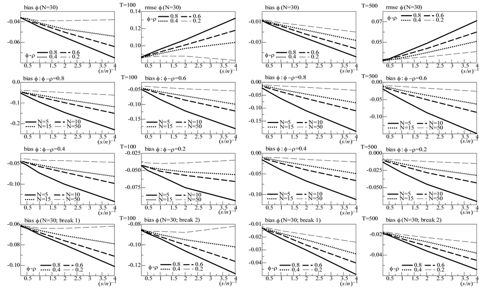
Figure 1. In the figure, Monte Carlo bias and RMSE statistics for the autoregressive parameter (f) are plotted for the case of no breaks (top and center plots) and one (break 1) and two (break 2) breaks (bottom plots), and a conditionally heteroskedastic common I(0) factor. Results are reported for various values of the persistence spread f ‒ ρ (0.2, 0.4, 0.6, 0.8) against various values of the (inverse) signal to noise ratio (s/n)−1 (4, 2, 1, 05, 0.25). The sample size T is 100 and 500 observations, the number of cross-sectional units N is 30, and the number of replications for each case is 2000. For the no breaks case, Monte Carlo bias statistics are also reported for other sample sizes N (5, 10, 15, 50) (center plots).
tional heteroskedasticity, for reasons of space, only the heteroskedastic case is discussed. Moreover, only the results for the  case are reported for the integrated case, as similar results have been obtained for the
  case.14
4.1.1. The Structural Stability Case
As shown in Figure 5 (top plots 1-4), for a cross-sectional sample size N = 30 units, a negligible downward bias for the  parameter (on average across (inverse) signal to noise ratio values) can be noted (−0.02 and −0.03, for the non integrated and integrated case, respectively, and
  (top plots 1-2); −0.01 and −0.006, respectively, and
  (top plots 3-4)), decreasing as the serial correlation spread,
  or
or , or the sample size
  increase.
On the contrary, as shown in Figure 1 and Figure 3 (top plots 1 and 3), the downward bias in f is increasing with the degree of persistence of the common factor , the (inverse) signal to noise ratio s/n-1 , and the serial correlation spread,
  or
or , yet decreasing with the sample size
 .
.
For the non integrated case (Figure 1, plots 1 and 3), there are only few cases ( ) when a 10%, or larger, bias in
  is found, occurring when the series are particularly noisy
 ; for the stationary long memory case a 10% bias, or smaller, is found for
 , while for the non stationary long memory case for
  and a (relatively) large sample (
 ) (Figure 3, plots 1 and 3). Increasing the cross-sectional dimension
  yields improvements (see the next section).
Also, as shown in Figure 2 and Figure 4 (top plots 1-4), very satisfactory is the estimation of the unobserved common stochastic factor, as the  statistic is always below 0.2 (0.14 (0.10)), on average, for
  (
( ) for the non integrated case (Figure 2, top plots 2 and 4); 0.06 (0.03), on average, for
  (
( ) for the integrated case (Figure 4, top plots 2 and 4). Moreover, the correlation coefficient between

Figure 2. In the figure, Monte Carlo Carlo Theil’s index (IC) and correlation coefficient (Corr) statistics, concerning the estimation of the conditionally heteroskedastic common I(0) factor, are plotted for the case of no breaks (top and center plots) and one (break 1) and two (break 2) breaks (bottom plots). Results are reported for various values of the persistence spread f ‒ ρ (0.2, 0.4, 0.6, 0.8) against various values of the (inverse) signal to noise ratio (s/n)−1 (4, 2, 1, 05, 0.25). The sample size T is 100 and 500 observations, the number of cross-sectional units N is 30, and the number of replications for each case is 2000. For the no breaks case, Monte Carlo correlation coefficient statistics are also reported for other sample sizes N (5, 10, 15, 50) (center plots).
the actual and estimated common factors is always very high, 0.98 and 0.99, on average, respectively, for both sample sizes (Figure 2 and Figure 4, top plots 1 and 3).
Results for smaller and larger cross-sectional samples. In Figures 1-4 (center plots, i.e., rows 2 and 3), the bias for the  parameter and the correlation coefficient between the actual and estimated common factors are also plotted for different cross-sectional dimensions, i.e.,
  , for the non integrated and integrated cases, respectively; statistics for the
  parameter are not reported, as the latter is always unbiasedly estimated, independently of the cross-sectional dimension.
As is shown in the plots, the performance of the estimator crucially depends on ,
,  , and
, and .
.
For the non integrated case (Figure 1), when the (inverse) signal to noise ratio is low, i.e.,  the downward bias is already mitigated by using a cross-sectional sample size as small as
 , for
, for
 ; as
; as  increases, similar results are obtained for higher
 , i.e.,
  and
and , or
, or
 and
and  (center plots, column 1-2). For a larger sample size, i.e.,
  (center plotscolumn 3-4), similar conclusions hold, albeit for the
  the (inverse) signal to noise ratio can be higheri.e.,
 ; similarly for
  with
with .
.
For the integrated case (Figure 3) conditions are slightly more restrictive; in particular, for the stationary long memory case, when the (inverse) signal to noise ratio is low, i.e.,  , the downward bias is already mitigated by setting
  and
and ; similar results are obtained for higher
  and N, i.e.,
  and
and , or
, or  and
and  (center plots, column 1-2). Similar conclusions can be drawn for
  (center plots, column 3-4), albeit, holding
  constant, accurate estimation is

Figure 3. In the figure, Monte Carlo bias statistics for the autoregressive parameter (f) are plotted for the case of no breaks (top and center plots) and one (break 1) and two (break 2) breaks (center and bottom plots), and a conditionally heteroskedastic common I(d) factor ( ). Results are reported for various values of the persistence spread d − ρ (0.2, 0.4, 0.6, 0.8, 1) against various values of the (inverse) signal to noise ratio (s/n)−1 (4, 2, 1, 05, 0.25). The sample size T is 100 and 500 observations, the number of cross-sectional units N is 30, and the number of replications for each case is 2000. For the no breaks case, Monte Carlo bias statistics are also reported for other sample sizes N (5, 10, 15, 50) (center plots).
obtained also for higher . Similarly also for the non stationary case (long memory or
 ); yet, holding
  constant, either larger
 , or lower
 , would be required for accurate estimation.
Coherently, the correlation coefficients between the actual and estimated common factors (Figure 2 and Figure 4, center plots) point to satisfactory estimation (a correlation coefficient higher than 0.9) also in the case of a small temporal sample size, provided the (inverse) signal to noise ratio is not too high, and/or the cross-sectional dimension is not too low  and
and ;
;  and
and ;
;  and
and ).
).
4.1.2. The Structural Change Case
While concerning the estimation of the  parameter no sizable differences can be found for the designs with structural change, relatively to the case of structural stability15, the complexity of the break process may on the other hand affect estimation accuracy for the
  parameter, worsening as the number of break points increases, particularly when the temporal sample size is small (
 ).
).
Yet, for the no integration case (Figure 1, bottom plots), already for  the performance is very satisfactory for both designs, independently of the (inverse) signal to noise ratio
  (bottom plots, columns 3 and 4); on the contrary, for
  the performance is satisfactory (at most a 10% bias) only when the series are not too noisy (
 ) (bottom plots, columns 1 and 2). Also, similar to the structural stability case, the (downward) bias in the
  parameter is increasing with the degree of persistence of the common factor d, the (inverse) signal to noise ratio
 , and
, and  or
or , yet decreasing with the sample size
 .
.
Coherent with the above results, satisfactory estimation of the unobserved common stochastic factor (Figure 2, bottom plots) and break process can also be noted (Figure 5, bottom plots, columns 1 and 3); for

Figure 4. In the figure, Monte Carlo Carlo correlation coefficient (Corr) statistics, concerning the estimation of the conditionally heteroskedastic common I(d) factor ( ), are plotted for the case of no breaks (top and center plots) and one (break 1) and two (break 2) breaks (bottom plots). Results are reported for various values of the persistence spread d − ρ (0.2, 0.4, 0.6, 0.8, 1) against various values of the (inverse) signal to noise ratio (s/n)−1 (4, 2, 1, 05, 0.25). The sample size T is 100 and 500 observations, the number of cross-sectional units N is 30, and the number of replications for each case is 2000. For the no breaks case, Monte Carlo correlation coefficient statistics are also reported for other sample sizes N (5, 10, 15, 50) (center plots).
the common stochastic factor, the ic statistic (not reported) is in fact always below 0.2 for  (0.11 and 0.13, on average, for the single break point and two-break points case, respectively) and below 0.3 for
  (0.17 and 0.20, on average; column 1), while the actual and estimated common stochastic factors are strongly correlated: for
  (
( ), on average, the correlation coefficient is 0.96 (0.98) for the single breakpoint case and 0.93 (0.97) for the two-break points case (column 3).
Very accurate is also the estimation of the common break process: the IC statistic is never larger than 0.15 for  and 0.075 for
  (Figure 5, bottom plots, columns 1 and 3), while the correlation coefficient is virtually 1 for the single break case and never below 0.96 for
  and 0.99 for
  for the two-break points case (not reported). Given the assumption of known break points, the performance in terms of correlation coefficient is not surprising; yet, the very small Theil’s index is indicative of success in recovering the changing level of the unobserved common break process.
Concerning the integrated case, some differences relatively to the nonintegrated case can be noted; as shown in Figure 5 (bottom plots, columns 2 and 4), albeit the overall recovery of the common break process is always very satisfactory across the various designs, independently of the sample size (the IC statistic is never larger than 0.14; bottom plots), performance slightly worsens as the complexity of the break process and persistence intensity (d ) increase: the average correlation coefficient between the estimated and actual break processes (center plots) falls from 1 when  (single break point case) to 0.93 when
  (two-break points case).
Moreover, concerning the estimation of the common stochastic factor (Figure 4, center and bottom plots, columns 1-4), for the covariance stationary case ( ) results are very close to the non integrated case, i.e., an IC statistic (not reported) always below 0.2 for
  (0.12 and 0.14, on average, for the single break point and two-break points case, respectively) and below 0.3 for
  (0.21 and 0.24, on average, respectively); the correlation coefficient is also very high: 0.94 and 0.91, on average,
  (columns 1
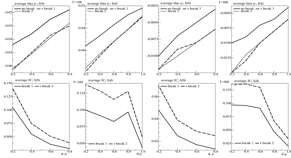
Figure 5. In the figure, average Monte Carlo statistics (across values for the inverse signal to noise ratio) for the bias in the autoregressive idiosyncratic parameter (ρ) (top plots) and Theil’s index (IC) statistic for the common break process (bottom plots) are plotted for the non integrated (I(0)) and integrated (I(d), ) cases. Results are reported for various values of the persistence spreads f − ρ (0.2, 0.4, 0.6, 0.8) and d − ρ (0.2, 0.4, 0.6, 0.8, 1). The sample size T is 100 and 500 observations, the number of cross-sectional units N is 30, and the number of replications for each case is 2000.
and 2); 0.97 and 0.96, on average,  (columns 3 and 4).
On the contrary, for the non stationary case performance is worse, showing average IC statistics (not reported) of 0.32 (0.32) and 0.42 (0.44), respectively, for the single break point (center plots) and two-break points (bottom plots) case and  (
( ); the average correlation coefficient is 0.79 (0.78) and 0.68 (0.66), respectively. Coherently, a worsening in the estimation of the common factor autoregressive parameter
 , for the
  and
and  case, can be noted (Figure 3, center and bottom plots), while comparable results to the short memory case can be found for
 . The latter findings are however not surprising, as the stronger the degree of persistence of the stochastic component (and of the series, therefore) and the less accurate the disentangling of the common break and break-free parts can be expected; overall, Monte Carlo results point to accurate decompositions also for the case of moderate nonstationary long memory, albeit deterioration in performance becomes noticeable.
5. Conclusion
In the paper, a general strategy for large-scale modeling of macroeconomic and financial data, set within the factor vector autoregressive model (F-VAR) framework is introduced. The proposed approach shows minimal pretesting requirements, performing well independently of integration properties of the data and sources of persistence, i.e., deterministic or stochastic, accounting for common features of different kinds, i.e., common integrated (of the fractional or integer type) or non integrated stochastic factors, also heteroskedastic, and common deterministic break processes. Consistent and asymptotically normal estimation is performed by means of QML, implemented through an iterative multi-step algorithm. Monte Carlo results strongly support the proposed approach. Empirical implementations can be found in [37] [67] -[69] , showing the approach being easy to implement and effective also in the case of very large systems of dynamic equations.
Acknowledgements
A previous version of the paper was presented at the 19th and 21st Annual Symposium of the Society for Non Linear Dynamics and Econometrics, the 4th and 6th Annual Conference of the Society for Financial Econometrics, the 65th European Meeting of the Econometric Society (ESEM), the 2011 NBER-NSF Time Series Conference, the 5th CSDA International Conference on Computational and Financial Econometrics. The author is grateful to conference participants, N. Cassola, F. C. Bagliano, C. Conrad, R. T. Baillie, J. Bai, for constructive comments. This project has received funding from the European Union’s Seventh Framework Programme for research, technological development and demonstration under grant agreement no. 3202782013-2015 and PRINMIUR 2009.
As Mitsuo Aida wrote in one of his poems, somewhere in life/there is a path/that must be taken regardless of how hard we try to avoid it/at that time, all one can do is remain silent and walk the path/neither complaining nor whining/saying nothing and walking on/just saying nothing and showing no tears/it is then/as human beings, /that the roots of our souls grow deeper. This paper is dedicated to the loving memory of A.
References
- Stock, J.H. and Watson, M.W. (2011) Dynamic Factor Models. In: Clements, M.P. and Hendry, D.F., Eds., Oxford Handbook of Economic Forecasting, Oxford University Press, Oxford, 35-60.
- Geweke, J. (1977) The Dynamic Factor Analysis of Economic Time Series. In: Aigner, D.J. and Goldberger, A.S., Eds., Latent Variables in Socio-Economic Models 1, North-Holland, Amsterdam.
- Dees, S., Pesaran, M.H., Smith, L.V. and Smith, R.P. (2010) Supply, Demand and Monetary Policy Shocks in a Multi-Country New Keynesian Model. ECB Working Paper Series, No. 1239.
- Bai, J. and Ng, S. (2004) A Panic Attack on Unit Roots and Cointegration. Econometrica, 72, 1127-1177.
- Bai, J.S. (2003) Inferential Theory for Factor Models of Large Dimensions. Econometrica, 71, 135-171. http://dx.doi.org/10.1111/1468-0262.00392
- Bai, J.S. and Perron, P. (1998) Testing for and Estimation of Multiple Structural Changes. Econometrica, 66, 47-78. http://dx.doi.org/10.2307/2998540
- Hamilton, J.D. (1989) A New Approach to the Economic Analysis of Nonstationary Time Series and the Business Cycle. Econometrica, 57, 357-384. http://dx.doi.org/10.2307/1912559
- Enders, W. and Lee, J. (2012) The Flexible Fourier Form and Dickey-Fuller Type Unit Root Tests. Economics Letters, 117, 196-199. http://dx.doi.org/10.1016/j.econlet.2012.04.081
- Baillie, R.T. and Morana, C. (2009) Modeling Long Memory and Structural Breaks in Conditional Variances: An Adaptive FIGARCH Approach. Journal of Economic Dynamics and Control, 33, 1577-1592. http://dx.doi.org/10.1016/j.jedc.2009.02.009
- Baillie, R.T. and Morana, C. (2012) Adaptive ARFIMA Models with Applications to Inflation. Economic Modelling, 29, 2451-2459. http://dx.doi.org/10.1016/j.econmod.2012.07.011
- González, A. and Teräsvirta, T. (2008) Modelling Autoregressive Processes with a Shifting Mean. Studies in Nonlinear Dynamics and Econometrics, 12, 1558-3708. http://dx.doi.org/10.2202/1558-3708.1459
- Engle, R.F. and Rangel, J.C. (2008) The Spline-GARCH Model for Low Frequency Volatility and Its Global Macroeconomic Causes. Review of Financial Studies, 21, 1187-1222. http://dx.doi.org/10.1093/rfs/hhn004
- Beran, J. and Weiershauser, A. (2011) On Spline Regression under Gaussian Subordination with Long Memory. Journal of Multivariate Analysis, 102, 315-335. http://dx.doi.org/10.1016/j.jmva.2010.09.007
- Beran, J. and Feng, Y.H. (2002) SEMIFAR Models—A Semiparametric Approach to Modelling Trends, Long-Range Dependence and Nonstationarity. Computational Statistics and Data Analysis, 40, 393-419. http://dx.doi.org/10.1016/S0167-9473(02)00007-5
- Engle, R.F. and Smith, A.D. (1999) Stochastic Permanent Breaks. The Review of Economics and Statistics, 81, 553-574. http://dx.doi.org/10.1162/003465399558382
- Ray, B.K. and Tsay, R.S. (2002) Bayesian Methods for Change-Point Detection in Long-Range Dependent Processes. Journal of Time Series Analysis, 23, 687-705. http://dx.doi.org/10.1111/1467-9892.00286
- Lu, Y. and Perron, P. (2010) Modeling and Forecasting Stock Return Volatility Using a Random Level Shift Model. Journal of Empirical Finance, 17, 138-156. http://dx.doi.org/10.1016/j.jempfin.2009.10.001
- Perron, P. and Varsnekov, R.T. (2012) Combining Long Memory and Level Shifts in Modeling and Forecasting the Volatility of Asset Returns. Boston University, Boston.
- Chapman, D.A. and Ogaki, M. (1998) Cotrending and the Stationarity of the Real Interest Rate. Economics Letters, 42, 133-138. http://dx.doi.org/10.1016/0165-1765(93)90050-M
- Bierens, H.J. (2000) Nonparametric Nonlinear Cotrending Analysis, with an Application to Interest and Inflation in the United States. Journal of Business and Economic Statistics, 18, 323-337. http://dx.doi.org/10.2307/1392265
- Hendry, D.F. (1996) A Theory of Co-Breaking. Nuffield College, University of Oxford, Oxford.
- Hendry, D.F. and Massmann, M. (2007) Co-Breaking: Recent Advances and a Synopsis of the Literature. Journal of Business and Economic Statistics, 25, 33-51. http://dx.doi.org/10.1198/073500106000000422
- Engle, R.F. and Kozicki, S. (1993) Testing for Common Features. Journal of Business & Economic Statistics, 11, 369-380. http://dx.doi.org/10.1080/07350015.1993.10509966
- Engle, R.F. and Granger, C. (1987) Co-Integration and Error Correction: Representation, Estimation and Testing. Econometrica, 55, 251-276. http://dx.doi.org/10.2307/1913236
- Bollerslev, T. (1990) Modelling the Coherence in Short-Run Nominal Exchange Rates: A Multivariate Generalized Arch Approach. Review of Economics and Statistics, 72, 489-505. http://dx.doi.org/10.2307/2109358
- Baillie, R.T., Bollerslev, T. and Mikkelsen, H.O. (1996) Fractionally Integrated Generalized Autoregressive Conditional Heteroskedasticity. Journal of Econometrics, 74, 3-30. http://dx.doi.org/10.1016/S0304-4076(95)01749-6
- Conrad, C. and Haag, B.R. (2006) Inequality Constraints in the Fractionally Integrated GARCH Model. Journal of Financial Econometrics, 4, 413-449. http://dx.doi.org/10.1093/jjfinec/nbj015
- Chan, N.H. and Palma, W. (1998) State Space Modeling of Long Memory Processes. Annals of Statistics, 26, 719-740. http://dx.doi.org/10.1214/aos/1028144856
- Kilian, L. (2011) Structural Vector Autoregressions. CEPR Discussion Paper, No. 8515.
- Beran, J. and Feng, Y.H. (2001) Local Polynomial Estimation with a FARIMA-GARCH Error Process. Bernoulli, 7, 733-750. http://dx.doi.org/10.2307/3318539
- Beran, J. and Feng, Y.H. (2002) Data Driven Bandwidth Choice for SEMIFAR Models. Journal of Computational and Graphical Statistics, 11, 690-713. http://dx.doi.org/10.1198/106186002420
- Bordignon, S. and Raggi, D. (2010) Long Memory and Nonlinearities in Realized Volatility. University of Padova, Padova.
- Martens, M., van Dijk, D. and de Pooter, M. (2003) Modeling and Forecasting S&P500 Volatility: Long Memory, Structural Breaks and Nonlinearity. Erasmus University of Rotterdam, Rotterdam.
- Grassi, S. and de Magistris, P.S. (2011) When Long Memory Meets the Kalman Filter: A Comparative Study. Aarhus University, Aarhus.
- Lavielle, M. and Moulines, E. (2000) Least-Squares Estimation of an Unknown Number of Shifts in a Time Series. Journal of Time Series Analysis, 21, 33-59. http://dx.doi.org/10.1111/1467-9892.00172
- Granger, C.W.J. and Hyung, N. (2004) Occasional Structural Breaks and Long Memory with an Application to the S&P500 Absolute Returns. Journal of Empirical Finance, 11, 399-421. http://dx.doi.org/10.1016/j.jempfin.2003.03.001
- Morana, C. (2014) New Insights on the US OIS Spreads Term Structure during the Recent Financial Turmoil. Applied Financial Economics, 24, 291-317. http://dx.doi.org/10.1080/09603107.2013.864034
- Bai, J.S. and Ng, S. (2013) Principal Components Estimation and Identification of Static Factors. Journal of Econometrics, 176, 18-29. http://dx.doi.org/10.1016/j.jeconom.2013.03.007
- Robin, J.M. and Smith, R.J. (2000) Tests of Rank. Econometric Theory, 16, 151-175. http://dx.doi.org/10.1017/S0266466600162012
- Peres-Neto, P.R., Jackson, D.A. and Somers, K.M. (2005) How Many Principal Components? Stopping Rules for Determining the Number of Non-Trivial Axes Revisited. Computational Statistics and Data Analysis, 49, 974-997. http://dx.doi.org/10.1016/j.csda.2004.06.015
- Bai, J. and Ng, S. (2002) Determining the Number of Factors in Approximate Factor Models. Econometrica, 70, 191-221. http://dx.doi.org/10.1111/1468-0262.00273
- Bai, J.S. and Ng, S. (2007) Determining the Number of Primitive Shocks in Factor Models. Journal of Business and Economic Statistics, 25, 52-60. http://dx.doi.org/10.1198/073500106000000413
- Nielsen, M.O. and Frederiksen, P.H. (2005) Finite Sample Comparison of Parametric, Semiparametric and Wavelet Estimators of Fractional Integration. Econometric Reviews, 24, 405-443. http://dx.doi.org/10.1080/07474930500405790
- Chan, N.H. and Palma, W. (2006) Estimation of Long-Memory Time Series Models: A Survey of Different Likelihood Based Approaches. In: Fomby, T.H. and Terrel, D., Eds., Econometric Analysis of Economic and Financial Time Series, Advances in Econometrics, Vol. 20, Emerald Group Publishing Limited, Bingley, 89-121.
- Robinson, P.M. (2006) Conditional-Sum-of-Squares Estimation of Models for Stationary Time Series with Long Memory. IMS Lecture Notes-Monograph Series, Time Series and Related Topics, 52, 130-137. http://dx.doi.org/10.1214/074921706000000996
- Sowell, F. (1992) Maximum Likelihood Estimation of Stationary Univariate Fractionally Integrated Time Series Models. Journal of Econometrics, 53, 165-188. http://dx.doi.org/10.1016/0304-4076(92)90084-5
- Martin, L.V. and Wilkins, N.P. (1999) Indirect Estimation of ARFIMA and VARFIMA Models. Journal of Econometrics, 93, 149-175. http://dx.doi.org/10.1016/S0304-4076(99)00007-x
- Baillie, R. and Kapetanios, G. (2013) Inference for Impulse Response Functions from Multivariate Strongly Persistent Processes. Queen Mary University of London, London.
- Bai, J.S. and Ng, S. (2006) Confidence Intervals for Diffusion Index Forecasts and Inference with Factor-Augmented Regressions. Econometrica, 74, 1133-1150. http://dx.doi.org/10.1111/j.1468-0262.2006.00696.x
- Bai, J.S. and Ng, S. (2008) Forecasting Economic Time Series Using Targeted Predictors. Journal of Econometrics, 146, 304-317. http://dx.doi.org/10.1016/j.jeconom.2008.08.010
- Granger, C.W.J. and Jeon, Y. (2004) Thick Modeling. Economic Modelling, 21, 323-343.
- Alexander, C.O. (2002) Principal Component Models for Generating Large GARCH Covariance Matrices. Economic Notes, 31, 337-359. http://dx.doi.org/10.1111/1468-0300.00089
- Amado, C. and Terasvirta, T. (2008) Modelling Conditional and Unconditional Heteroskedasticity with Smoothly Time-Varying Structure. CREATES Research Paper, No. 8.
- Hamilton, J.D. and Susmel, R. (1994) Autoregressive Conditional Heteroskedasticity and Changes in Regime. Journal of Econometrics, 64, 307-333. http://dx.doi.org/10.1016/0304-4076(94)90067-1
- Engle, R.F. (2002) Dynamic Conditional Correlation—A Simple Class of Multivariate GARCH Models. Journal of Business and Economic Statistics, 20, 339-350. http://dx.doi.org/10.1198/073500102288618487
- Engle, R.F. and Kelly, B.T. (2012) Dynamic Equicorrelation. Journal of Business and Economics Statistics, 30, 212-228.
- Quah, D. and Sargent, T.J. (1992) A Dinamic Index Model for Large Cross-Section. In: Stock, J. and Watson, M., Eds., Business Cycle, University of Chicago Press, Chicago.
- Watson, M. and Engle, R.F. (1983) Alternative Algorithms for the Estimation of Dynamic Factor, Mimic and Varying Coefficient Regression Models. Journal of Econometrics, 23, 385-400. http://dx.doi.org/10.1016/0304-4076
- Doz, C., Giannone, D. and Reichlin, L. (2011) A Two-Step Estimator for Large Approximate Dynamic Factor Models Based on Kalman Filtering. Journal of Econometrics, 164, 188-205. http://dx.doi.org/10.1016/j.jeconom.2011.02.012
- Doz, C., Giannone, D. and Reichlin, L. (2012) A Quasi Maximum Likelihood Approach for Large Approximate Dynamic Factor Models. Review of Economics and Statistics, 94, 1014-1024. http://dx.doi.org/10.1162/REST_a_00225
- Bai, J.S. (2004) Estimating Cross-Section Common Stochastic Trends in Nonstationary Panel Data. Journal of Econometrics, 122, 137-138. http://dx.doi.org/10.1016/j.jeconom.2003.10.022
- Castells, F., Laguna, P., Sornmo, L., Bollmann, A. and Millet-Roig, J. (2007) Principal Component Analysis in ECG Signa Processing. EURASIP Journal on Advances in Signal Processing, 1, 98-119. http://dx.doi.org/10.1155/2007/74580
- Morana, C. (2007) Multivariate Modelling of Long Memory Processes with Common Components. Computational Statistics and Data Analysis, 52, 919-934. http://dx.doi.org/10.1016/j.csda.2006.12.010
- Hatanka, M. and Yamada, H. (1994) Co-Trending: An Extended Version. University of Hiroshima, Hiroshima.
- Lansang, J.R.G. and Barrios, E.B. (2009) Principal Components Analysis of Nonstationary Time Series Data. Statistics and Computing, 19, 173-187. http://dx.doi.org/10.1007/s11222-008-9082-y
- Morana, C. (2014) Factor Vector Autoregressive Estimation of Heteroskedastic Persistent and Non Persistent Processes Subject to Structural Breaks. DEMS Working Paper Series, No. 273.
- Cassola, N. and Morana, C. (2012) Euro Money Market Spreads during the 2007-? Financial Crisis. Journal of Empirical Finance, 19, 548-557. http://dx.doi.org/10.1016/j.jempfin.2012.04.003
- Morana, C. (2013) Oil Price Dynamics, Macro-Finance Interactions and the Role of Financial Speculation. Journal of Banking and Finance, 37, 206-226. http://dx.doi.org/10.1016/j.jbankfin.2012.08.027
- Bagliano, F.C. and Morana, C. (2014) Determinants of US Financial Fragility Conditions. Research in International Business and Finance, 30, 377-392. http://dx.doi.org/10.1016/j.ribaf.2012.08.003
NOTES

*The literature on F-VAR models is large. See for a survey.

2Monte Carlo evidence reported in suggests that the truncation lag should increase with the sample size and the complexity of the ARFIMA representation of the long memory process, still remaining very small relatively to the sample size. For instance, for the covariance stationary fractional white noise case and a sample of 100 observations truncation can be set as low as 6 lags, while for a sample of 10,000 observations it should be increased to 14 lags; for the case of a covariance stationary ARFIMA (1,d,1) process and a sample of 1000 observations truncation may be set to 30 lags. See for further details.

3See for a recent survey.

4The orthogonality of  and
and  can however also be imposed when jointly estimating the deterministic and stochastic components by means of augmented ARFIMA models.
5The strong consistency of the  estimator of the break fraction, independently of the rate of decay of the autocovariance function of the error process, has been proved in when the number of break points is known; a modified Bayes-Schwarz selection criterion for the number of break points is also proposed.

6Alternatively,  can be obtained by regressing
  on
on  (and the initial estimate
 ), using OLS.

7Alternatively, the new break-free process can be computed as .
.
8Alternatively,  can be obtained by regressing
  on
on  and the updated estimate
 , using OLS. This would also yield a new estimate
  to be used in the computation of the updated gap vector.
9For instance, the procedure can be stopped when , where the objective function is written as in (26).
10See and for a survey of alternative estimators of the fractional differencing parameter.
11Depending on the parametric structure, system estimation may however become unfeasible when the number of factors is too large.

12In particular, under some general conditions, given any invertible matrix ,
,  consistency and asymptotic normality of PCA for
 , at each point in time, is established for
  and
and  and the case of
  unobserved factors and idiosyncratic components, the latter also displaying limited heteroskedasticity in both their time-series and cross-sectional dimensions ; for 𝑁,𝑇→∞ and 𝑁𝑇
3
→0 and the case of  (non cointegrated) unobserved factors and
  idiosyncratic components, similarly showing limited heteroskedasticity in both the time-series and cross-sectional dimensions (). The latter result is actually obtained by applying PCA to the level of the series, rather than their first differences. Moreover, for both the
  and
and  case,
case,  consistency and asymptotic normality of PCA for
  is established under the same conditions, as well as
  consistency and asymptotic normality of PCA for the unobserved common components
 , at each point in time, for
 .
.
The conditions for consistency and asymptotic normality reported in and implicitly cover also the case in which PCA is implemented using the estimated break  and break-free
  components, rather than the observed
𝑥
𝑡
series; in fact, by assuming  and
and , then
  and
and , which are static factor structures as assumed in and . It appears that assumption E in , page 143, i.e., weak dependence and limited cross-sectional correlation, holding for both noise (estimation error) components
  and
and , augmented with the assumption of their contemporaneous orthogonality, i.e.,
  , is then sufficient for the validity of PCA also when implemented on noisy data. In this respect PCA acts as noise suppressor: intuitively, PCs associated with the smallest eigenvalues are noise, which should be neglected when estimating the common factors. PCA estimation of the signal component can actually be shown to be optimal in terms of minimum mean square error [62].
13The use of PCA for the estimation of common deterministic trends has previously been advocated by . See also for applications to nonstationary data.

14Detailed results are available in the working paper version of this paper or upon request from the author.

15The average bias is −0.04 and −0.01, independent of the break process design and integration properties, when  and
and , respectively. Moreover, similar to the structural stability case the bias is decreasing as
 ,
,  , or the sample size
  increase, independent of the (inverse) signal to noise ratio.