Open Journal of Statistics
Vol. 2 No. 1 (2012) , Article ID: 16881 , 15 pages DOI:10.4236/ojs.2012.21008
Statistical Methods of SNP Data Analysis and Applications
1Faculty of Mathematics and Mechanics, Moscow State University, Moscow, Russia
2Faculty of Basic Medicine, Moscow State University, Moscow, Russia
Email: *ashashkin@hotmail.com
Received October 9, 2011; revised November 16, 2011; accepted November 20, 2011
Keywords: Genetic Data Statistical Analysis; Multifactor Dimensionality Reduction; Ternary Logic Regression; Random Forests; Stochastic Gradient Boosting; Independent Rule; Single Nucleotide Polymorphisms; Coronary Heart Disease; Myocardial Infarction
ABSTRACT
We develop various statistical methods important for multidimensional genetic data analysis. Theorems justifying application of these methods are established. We concentrate on the multifactor dimensionality reduction, logic regression, random forests, stochastic gradient boosting along with their new modifications. We use complementary approaches to study the risk of complex diseases such as cardiovascular ones. The roles of certain combinations of single nucleotide polymorphisms and non-genetic risk factors are examined. To perform the data analysis concerning the coronary heart disease and myocardial infarction the Lomonosov Moscow State University supercomputer “Chebyshev” was employed.
1. Introduction
In the last decade new high-dimensional statistical methods were developed for the data analysis (see, e.g., [1]). Special attention was paid to the study of genetic models (see, e.g., [2-4]). The detection of genetic susceptibility to complex diseases (such as diabetes and others) has recently drawn much attention in leading research centers. It is well-known that such diseases can be provoked by variations in different parts of the DNA code which are responsible for the formation of certain types of proteins. One of the most common individual’s DNA variations is a single nucleotide polymorphism (SNP), i.e. a nucleotide change in a certain fragment of genetic code (for some percentage of population). Quite a number of recent studies (see, e.g., [5,6] and references therein) support the paradigm that certain combinations of SNP can increase the complex disease risk whereas separate changes may have no dangerous effect.
There are two closely connected research directions in genomic statistics. The first one is aimed at the disease risk estimation assuming the genetic portrait of a person is known (in turn this problem involves estimation of disease probability and classification of genetic data into high and low risk domains). The second trend is to identify relevant combinations of SNPs having the most significant influence, either pathogenic or protective.
In this paper we propose several new versions of statistical methods to analyze multidimensional genetic data, following the above-mentioned research directions. The methods developed generalize the multifactor dimensionality reduction (MDR) and logic regression (LR). We employ also some popular machine learning methods (see, e.g., [2]) such as random forests (RF) and stochastic gradient boosting (SGB).
Ritchie et al. [7] introduced MDR as a new method of analyzing gene-gene and gene-environment interactions. Rather soon the method became very popular. According to [8], since the first publication more than 200 papers applying MDR in genetic studies were written.
LR was proposed by Ruczinski et al. in [9]. Further generalizations are given in [6,10] and other works. LR is based on the classical binary logistic regression and the exhaustive search for relevant predictor combinations. For genetic analysis it is convenient to use explanatory variables taking 3 values. Thus we employ ternary variables and ternary logic regression (TLR), whereas the authors of the above-mentioned papers employ binary ones.
RF and SGB were initiated by Breiman [11] and Friedman [12] respectively. They belong to ensemble methods which combine multiple predictions from a certain base algorithm to obtain better predictive power. RF and SGB were successfully applied to genetics data in a number of papers (see [2,13] and references therein).
We compare various approaches on the real datasets concerning coronary heart disease (CHD) and myocardial infarction (MI). Each approach (MDR, TLR and machine learning) is characterized by its own way of constructing disease prediction algorithms. For each method one or several prediction algorithms admitting the least estimated prediction error are found (a typical situation is that there are several ones with almost the same estimated prediction error). These prediction algorithms provide a way to determine the domains where the disease risk is high or low. It is also possible to select combinations of SNPs and non-genetic risk factors influencing the liability to disease essentially. Some methods allow to present such combinations immediately. Other ones, which employ more complicated forms of dependence between explanatory and response variables, need further analysis based on modifications of permutation tests. New software implementing the mentioned statistical methods has been designed and used.
This work was started in 2010 in the framework of the general MSU project headed by Professors V. A. Sadovnichy and V. A. Tkachuk (see [14]). MSU supercomputer “Chebyshev” was employed to perform data analysis.
The rest of the paper is organized as follows. In Section 2 we discuss various statistical methods and prove theorems justifying their applications. Section 3 is devoted to analysis of CHD and MI datasets. Section 4 contains conclusions and final remarks.
2. Methods
We start with some notation. Let  be the number of patients in the sample and let the vector
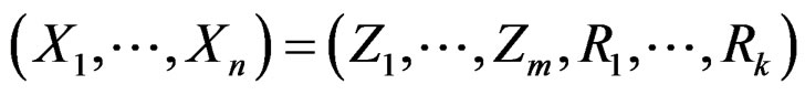
 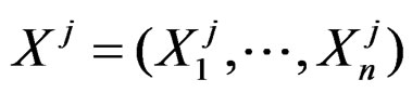 consist of genetic (SNP) and nongenetic risk factors of individual j
 . Here n is the total number of factors and
  is the value of the i-th variable (genetic or non-genetic factor) of individual j. These variables are called explanatory variables or predictors. If
  stands for a genetic factor (characterizes the i-th SNP of individual j) we set
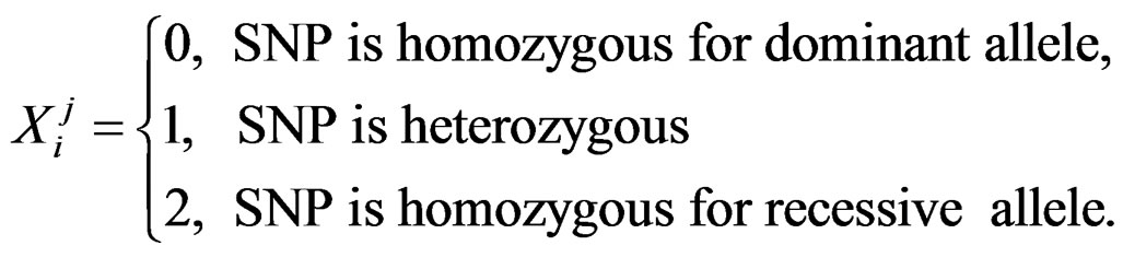
For biological background we refer, e.g., to [15].
We assume that non-genetic risk factors also take no more than three values, denoted by 0, 1 and 2. For example, we can specify a presence or absence of obesity (or hypercholesterolemia etc.) by the values 1 and 0 respectively. If a non-genetic factor takes more values (e.g., blood pressure), we can divide individuals into three groups according to its values.
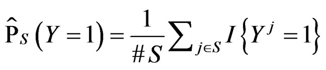
Further on  stand for genetic data and
  for non-genetic risk factors. Let a binary variable
  (response variable) be equal to 1 for a case, i.e. whenever individual j is diseased, and to –1 otherwise (for a control). Set

where

Suppose  are i.i.d. random vectors. Introduce a random vector
  independent of
  and having the same law as
 . All random vectors (and random variables) are considered on a probability space
  E denotes the integration w.r.t. P.
The main problem is to find a function in genetic and non-genetic risk factors describing the phenotype (that is the individual being healthy or sick) in the best way.
2.1. Prediction Algorithms
Let  denote the space of all possible values of explanatory variables. Any function
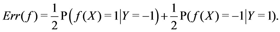
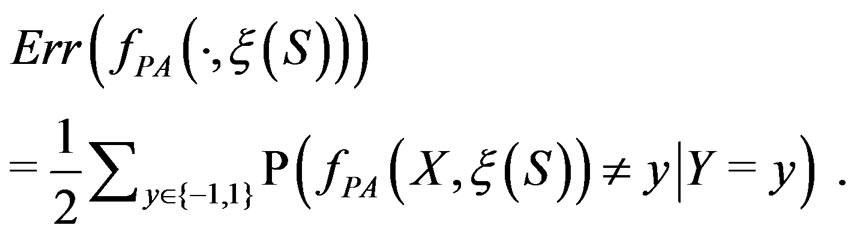
  is called a theoretical prediction function. Define the balanced or normalized prediction error for a theoretical prediction function
  as
as
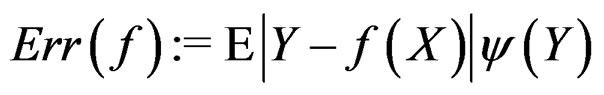
where the penalty function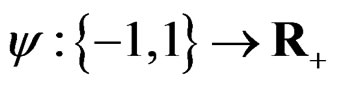 . Obviously
 (1)
(1)
Clearly  depends also on the law of
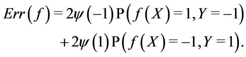
  but we simplify the notation. Following [8,16] we put
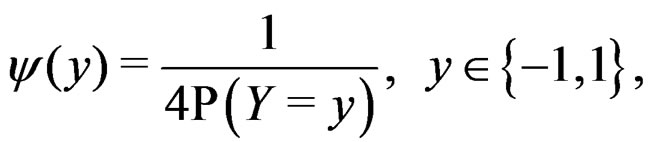
where the trivial cases  and
and  are excluded. Then
(2)
If  a sample is called balanced and one has
 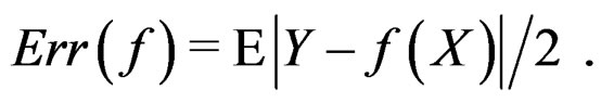 Therefore in this case
  equals the classification error
 . In general,
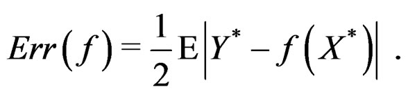
with  having the distribution

The reason to consider this weighted scheme is that a misclassification in a more rare class should be taken into account with a greater weight. Otherwise, if the probability of disease  is small, then the trivial function
  may have the least prediction error.
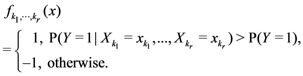
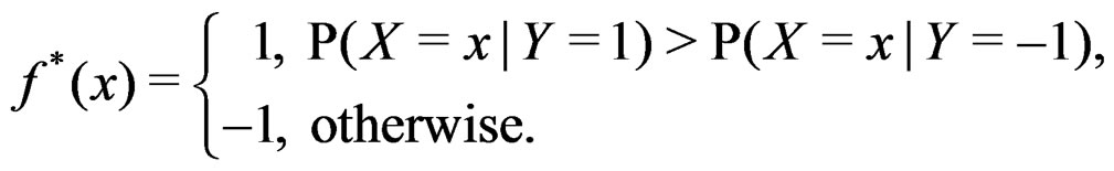
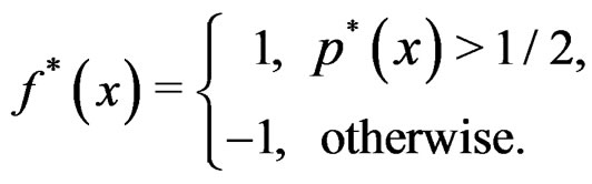
It is easy to prove that the optimal theoretical predicttion function minimizing the balanced prediction error is given by
 (3)
(3)
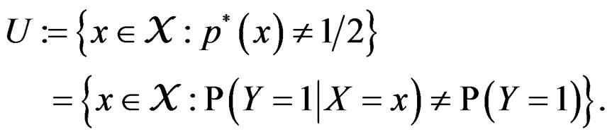
where
 (4)
(4)
Then each multilocus genotype (with added non-genetic risk factors)  is classified as high-risk if
  or low-risk if
Since  and
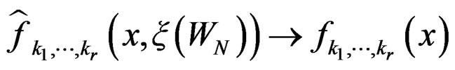
and  are unknown, the immediate application of (3) is not possible. Thus we try to find an approximation of unknown function
  using a prediction algorithm that is a function
with values in  which depends on
  and the sample
where
 (5)
(5)
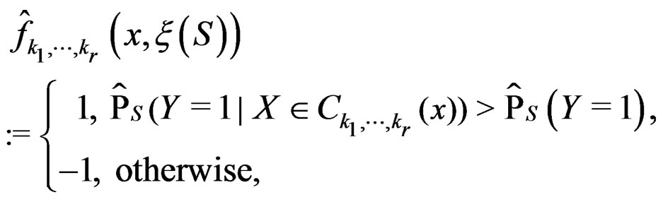
The simplest way is to employ formula (3) with  and
and  replaced by their statistical estimates. Consider
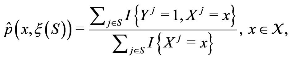 (6)
(6)
and take
 (7)
(7)
where  stands for the indicator of an event A and #D denotes the cardinality of a finite set D.
Along with (7) we consider
 (8)
(8)
for  Thus (6) is a special case of (8) for
  with
with . Note that a more difficult way is to search for the estimators of
  using several subsamples of
 .
.
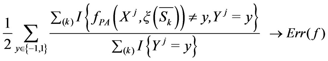
For a given prediction algorithm  keeping in mind (2), we set
 (9)
(9)
If one deals with too many parameters, overfitting is likely to happen, i.e. estimated parameters depend too much on the given sample. As a result the constructed estimates give poor prediction on new data. On the other hand, application of too simple model may not capture the studied dependence structure of various factors efficiently. However the trade-off between the model’s complexity and its predictive power allows to perform reliable statistical inference via new model validation techniques (see, e.g., [17]). The main tool of model selection is the cross-validation, see, e.g., [16]. Its idea is to estimate parameters by involving only a part of the sample (training sample) and afterwards use the remaining observations (test sample) to test the predictive power of the obtained estimates. Then an average over several realizations of randomly chosen training and test samples is taken, see [18].
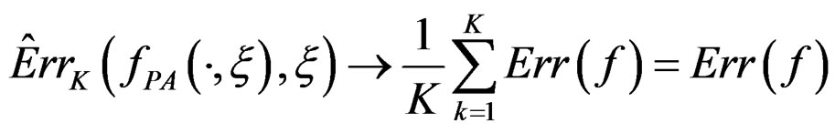
As the law of  is unknown, one can only construct an estimate
  of
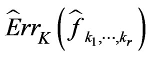
of  . In Section 3 we use the estimated prediction error
 (EPE) of a prediction algorithm
  which is based on K-fold cross-validation
  and has the form
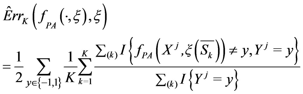 (10)
(10)
where the sum  is taken over j belonging to
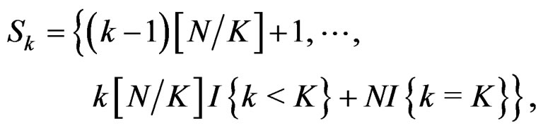 (11)
(11)
 and
and  is the integer part of
Let . Introduce

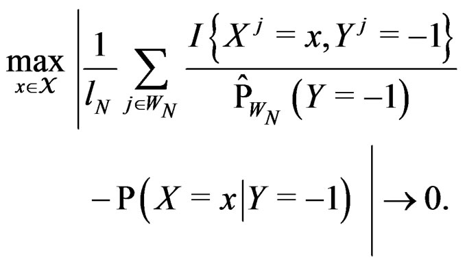
The next result provides wide sufficient conditions for consistency of estimate (10).
Theorem 1. Suppose there exist a subset  and a subset
  such that the following holds:
1) For each  and any finite dimensional vector v with components belonging to
  functions
  and f are constant on
 .
.
2) For each  and any
  with
with  one has
  a.s. when
 .
.
3)  if
if 
4) f is constant on .
.
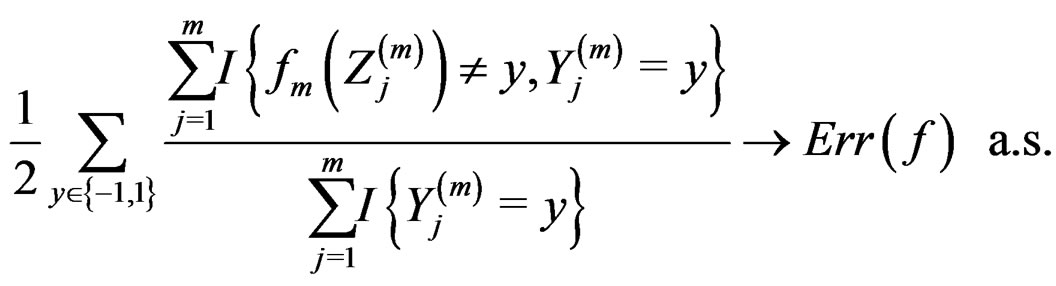
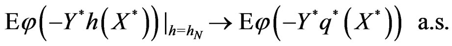
Then  a.s.,
a.s., .
.
Remark. If we replace condition 3 of Theorem 1 by a more restrictive assumption 3’) 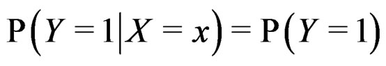 for all
  then we can take
  to remove condition 1.
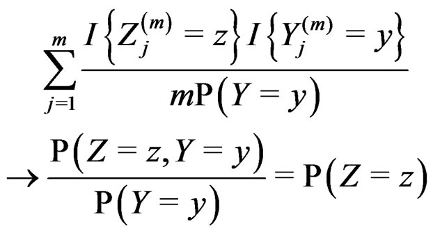
Proof. The proof is based on the following Lemma. Let  be an array of rowwise independent random elements distributed as
 , where Z takes values in a finite set
  and
and  takes values in
 . Assume that
 is an array of random variables with values in
 .
.
Suppose there exists  such that the following conditions hold:
1)  a.s. for all
 , as
, as , where a nonrandom function
 .
.
2)  if
if 
3)  is constant on
Then, as 
 (12)
(12)
Proof of Lemma. Set  and define events


Then the l.h.s. of (12) equals

For , we have
 (13)
(13)
The absolute value of the second term in the r.h.s. of (13) does not exceed  and tends to 0 a.s. if
 . This statement follows from the strong law of large numbers for arrays (SLLNA), see [19].
Note that
 (14)
(14)
According to SLLNA the first term in the r.h.s. of (14) goes to  a.s. We claim that the second term tends to 0 a.s. Indeed, the set
  is finite and the functions
 take only two values. Therefore, by condition 1, for almost all
 , there exists
  such that
  for all
  and
and . Hence second term in the r.h.s. of (14) equals 0 for all
 , which proves the claim. Thus, it remains to estimate the third term.
In view of condition 3, w.l.g. we may assume that  for
for  Then we obtain
 (15)
(15)
where
 .
.
SLLNA and condition 2 imply that, for  and
and  we have
almost surely. Therefore, for almost all  there exists
  such that
for all  and
and  Using the last estimate and (15) we finally get that, for
Hence  a.s. if
 . Combining (12)-(16) we obtain the desired result.
Let us return to the proof of Theorem 1. Fix  and take
where 
 ,
,  is introduced in (11), and x is any element of
  with
with  By condition 1 of Theorem 1,
  is well defined.
Applying Lemma to arrays
and , we obtain that almost surely
as  Thus
Thus
when  which completes the proof of Theorem 1.
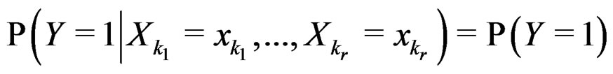
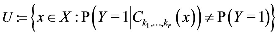
An important problem is to make sure that the predicttion algorithm  gives statistically reliable results. The quality of an algorithm is determined by its predicttion error (9) which is unknown and therefore the inference is based on consistent estimates of this error. Clearly the high quality of an algorithm means that it captures the dependence between predictors and response variables, so the error is made more rarely than it would be if these variables were independent. Consider a null hypothesis
  that
that  and
and  are independent. If they are in fact dependent, then for any reasonable prediction algorithm
  an appropriate test procedure involving
  should reject
  at the significance level
 , e.g., 5%. This shows that the results of the algorithm could not be obtained by chance. For such a procedure, we take a permutation test which allows to find the Monte Carlo estimate
 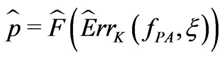 (see [20]) of the true p-value
 .
.
Here F is the cumulative distribution function (c.d.f.) of  under
under  and
and  is the corresponding empirical c.d.f. We reject
  if
if  For details we refer to [21].
Now we pass to the description of various statistical methods and their applications (in Section 3) to the cardiovascular risk detection.
2.2. Multifactor Dimensionality Reduction
MDR is a flexible non-parametric method of analyzing gene-gene and gene-environment interactions. MDR does not depend on a particular inheritance model. We give a rigorous description of the method following ideas of [7] and [8].
To calculate the balanced error of a theoretical predicttion function we use formula (2). Note that the approach based on penalty functions is not the only possible. Nevertheless it outperforms substantially other approaches involving overand undersampling (see [8]).
As mentioned earlier, the probability p(x) introduced in (4) is unknown. To find its estimate one can apply maximum likelihood approach assuming that the random variable  conditionally on
  has a Bernoulli distribution with unknown parameter
 . Then we come to (6).
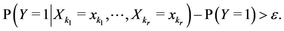
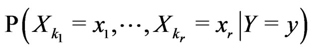
A direct calculation of estimate (6) with exhaustive search over all possible values of x is highly inefficient, since the number of different values of x grows exponentially with number of risk factors. Moreover, such a search leads to overfitting. Instead, it is usually supposed that  depends non-trivially not on all, but on certain variables xi. That is, there exist
  and a vector
  where
where  such that for each
  the following relation holds:
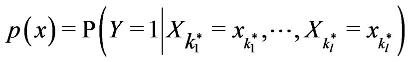 . (17)
In other words only few factors influence the disease and other ones can be neglected. A combination of indices 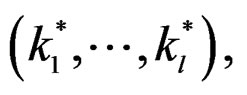 in formula (17) having minimal
  is called the most significant.
For  and indices
  set
set
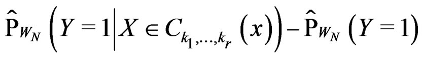
Consider the estimate
 (18)
(18)
where S is introduced in (5).
Theorem 2. Let  be the most significant combination. Then for any fixed
  one has 1)
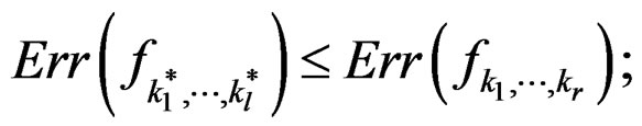
2)  is a strongly consistent asymptotically unbiased estimate of
  as
as 
3) for any  and all N large enough
 .
.
Proof. 1) It follows from (17) that  coinsides with function
  (see (3)) which has the minimal balanced prediction error.
2) Let us verify the conditions of Theorem 1 for 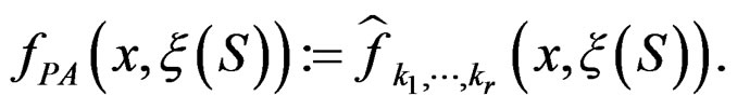 Condition 1 follows from the definition of
  Further, put
 (19)
(19)
where  was introduced in Section 2.1 before Theorem 1. We claim that, for each
  and any
  such that
 , the following relation holds:
 a.s. if
 .
.
Indeed, assume that, for some 
SLLNA implies that
converges a.s. to
 . Then, for almost all
  there exists
  such that

for all . Therefore, for all
 , we have
 , which proves the claim. Thus condition 2 of Theorem 1 is met.
Conditions 3 and 4 of Theorem 1 follow from (19) and the definitions of  and
and 
Since all conditions of Theorem 1 are satisfied, we have  a.s. and in mean (due to the Lebesgue theorem as
  is bounded by 1).
3) Follows from 1) and 2). 
In view of this result it is natural to pick one or a few combinations of factors with the smallest EPEs as an approximation for the most significant combination.
The last step in MDR is to determine statistical significance of the results. Here we test a null hypothesis of independence between predictors X and response variable Y. This can be done via the permutation test mentioned in Section 2.1.
MDR method with “independent rule”. We propose multifactor dimensionality reduction with “independent rule” (MDRIR) method to improve the estimate of probability . This approach is motivated by [22] which deals with classification of large arrays of binary data. The principal difficulty with employment of formula (6) is that the number of observations in numerator and denominator of the formula might be small even for large N (see, e.g., [23]). This can lead to inaccurate estimates and finally to a wrong prediction algorithm. Moreover, for some samples the denominator of (6) might equal zero.
The Bayes formula implies that  equals
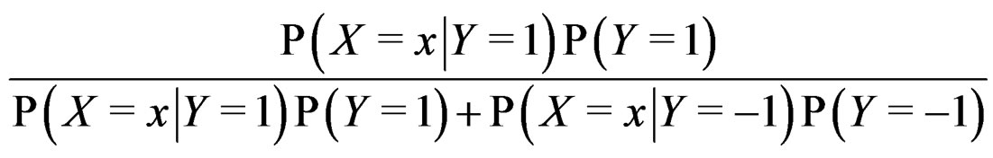
(20)
where the trivial cases  and
and  are excluded. Substituting (20) into (3) we obtain the following expression for the prediction function:
 (21)
(21)
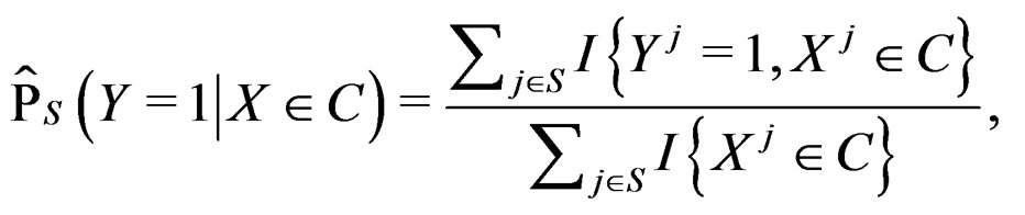
As in standard MDR method described above, we assume that formula (17) holds. It was proved in [22] that for a broad class of models (e.g., Bahadur and logit models) the conditional probability
where  can be estimated in the following way:
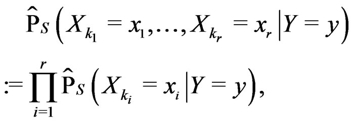 (22)
(22)
here (cf. (8))
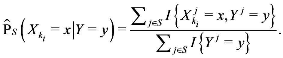 (23)
(23)
Combining (17) and (21)-(23) we find the desired estimate of 
A number of observations in numerator and denominator of (23) increases considerably comparing with (18). It allows to estimate the conditional probability more precisely whenever the estimate introduced in (22) is reasonable. For instance, sufficient conditions justifying the application of (22) are provided in [22, Cor.5.1]. MDRIR might have some advantage over MDR in case when the size l of the most significant combination  is large. However, MDR for small l can demonstrate better behavior than MDRIR.
Thus, as opposed to standard MDR method, MDRIR uses alternative estimates of conditional probabilities. All other steps (prediction algorithm construction, EPE calculation) remain the same. As far as we know, this modification of MDR has not been applied before. It is based on a combination of the original MDR method (see [7]) and the ideas of [22].
2.3. Ternary Logic Regression
LR is a semiparametric method detecting the most significant combinations of predictors as well as estimating the conditional probability of the disease.
Let  (where
 ) be the conditional probability of a disease defined in normalized sample, where
  was introduced in Section 2.1. Note that formula (3) can be written as follows:
We suppose that trivial situations when  do not occur and omit them from the consideration. To estimate
  we pass to the logistic transform
 (24)
(24)
where is the inverse logistic function. The logistic function equals
 ,
, Note that we are going to estimate the unknown disease probability with the help of linear statistics with appropriately selected coefficients. Therefore it is natural to avoid restrictions on possible values of the function estimated. Thus the logistic transform is convenient, as
  for
for  while
while  can take all real values.
Consider a class  of all real-valued functions in ternary variables
 . We call a model of the dependence between the disease and explanatory variables any subclass
 . Set
. Set
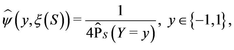
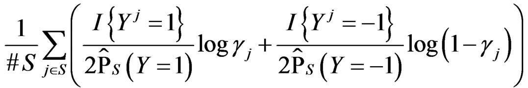
with  appearing in (7). Define the normalized smoothed score function
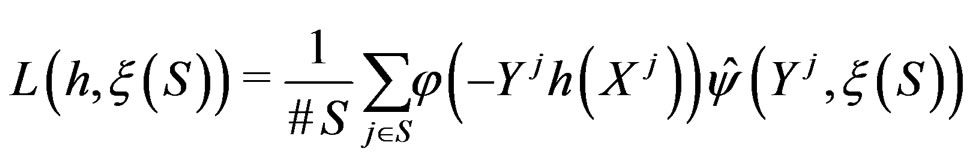 (25)
(25)
where S was introduced in (5), 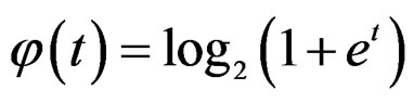 for
for  and
and . In contrast to previous works our version of LR (more precisely, TLR) scheme involves normalization (cf. (1)), i.e. taking the observations with weights dependent on the proportion of cases and controls in subsample
 . An easy computation yields that
  equals
  of the function
with 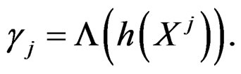 That is, minimizing the score function is equivalent to the normalized maximum likelihood estimation of
 .
.
The next theorem guarantees strong consistency of this estimation method whenever the model is correctly specified, i.e.  To formulate this result introduce
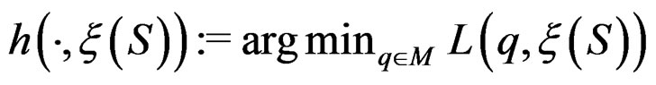 .
.
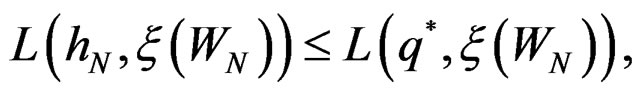
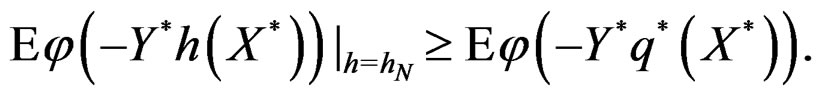
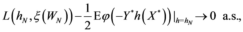
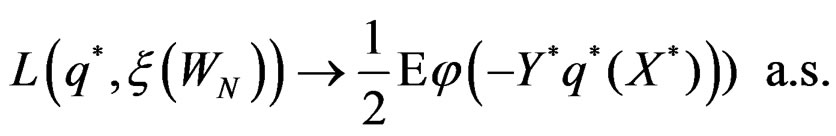
Theorem 3. Let 
 belong to M and
 .
.
Consider  and set
 .
.
Then  a.s. for all
  when
when . Moreover,
 a.s.,
a.s.,  where
where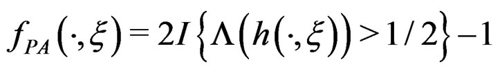 .
.
Proof. At first we show that
 a.s.
a.s.
for any  and all
  Put
Put  By definition
Using SLLNA, we get that a.s.
Obviously
These relations imply the desired estimate of . Similarly we prove that
for any  and all
 . Consequently, we see that
  for
for  here
here  and
and

If  then
then  is less than

By SLLNA, we get that
 a.s. (26)
uniformly over . Note also that
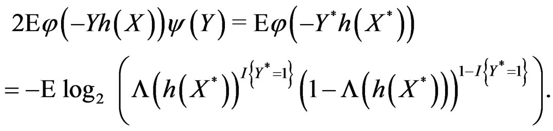
By the (conditional) information inequality,

attains its maximum over all functions h only at  introduced in (24). Under conditions of the theorem,
  Therefore, by definitions of
  and
and  we have
By (26) and SLLNA
Hence
This is possible only when  a.s. for all
  Indeed, for almost all
  we can always take a subsequence
  converging to some function
  with
with
Hence, by the information inequality, 
To establish the second part of Theorem 3 we note that converges a.s. to
 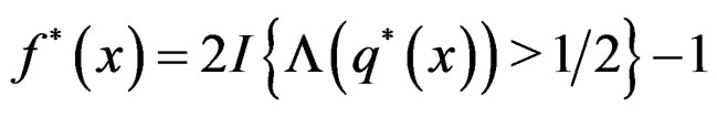 for all
  where
where
Then the conclusion follows from Remark after Theorem 1. The proof is complete.
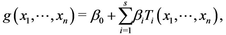
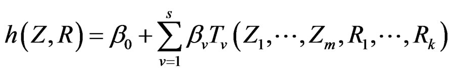
A wide and easy to handle class of models is obtained by taking functions linear in variables  or/and in their products. In turn these functions admit a convenient representation by elementary polynomials (EP). Recall that EP is a function T in ternary variables
  belonging to
  which can be represented as a finite sum of products
  where
where . The addition and multiplication of ternary variables is considered by modulo 3. Any EP can be represented as a binary tree in which knots (vertices which are not leaves) contain either the addition or multiplication sign, and each leaf corresponds to a variable. Different trees may correspond to the same EP, thus this relation is not one-to-one. However, it does not influence our problem, so we keep the notation T for a tree. A finite set of trees
  is called a forest. For a tree T its complexity C(T) is the number of leaves. The complexity C(F) of a forest F is the maximal complexity of trees constituting F. It is clear that if
  then there exists
  such that g has the form
 (27)
(27)
here  and
and  are EP.
Let us say that function g belongs to a class , where
 , if there exist a decomposition (27) of g such that all trees Ti (
 ) have complexity less or equal to r. We identify a function
  with pair
  where F is the corresponding forest and
  is the vector of coefficients in (27).
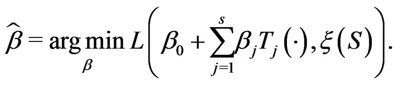
Minimization of  defined by (25) over all functions
  is done in two alternating steps. First, we find the optimal value of b while F is fixed (which is the minimization of a smooth function in several variables) and then we search for the best F. The main difficulty is to organize this search efficiently. Here one uses stochastic algorithms, since the number of such forests increases rapidly when the complexity r grows. For
 , a forest
  and a subsample
  (see (5)), consider a prediction algorithm
  setting
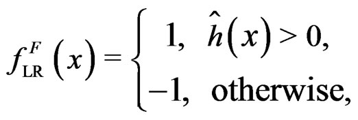
where  and
and
Define also the normalized prediction error of a forest  as
as .
.
A subgraph B of a tree T is called a branch if it is itself a binary tree (i.e. it can be obtained by selecting one vertex of T together with its offspring). The addition and multiplication signs standing in a knot of a tree are called operations, thus * stands for sum or product. Following [9], call the tree  a neighbor of T if it is obtained from T via one and only one of the following transformations.
1) Changing one variable to another in a leaf of the tree T (variable change).
2) Replacing an operation in a knot of a tree T with another one, i.e. sum to product or vice versa (operator change).
3) Changing a branch of two leaves to one of these leaves (deleting a leaf).
4) Changing a leaf to a branch of two leaves, one of which contains the same variable as in initial leaf (splitting a leaf).
5) Replacing a branch  with the branch
  (branch pruning).
6) Changing a branch B to a branch  (branch growing), here
  is a variable.
We say that forests F and  are neighbors if they can be written as
  and
and  where
where  and
and  are neighbors. The neighborhood relation defines a finite connected graph on all forests of equal size s with complexity not exceeding r. To each vertex F of this graph we assign a number
  To find the global minimum of a function defined on a finite graph we apply the simulated annealing method (see, e.g., [24]). This method constructs some specified Markov process which takes values in the graph vertices and converges with high probability to the global minimum of the function. To avoid stalling at a local minimal point the process is allowed to pass with some small probability to a point F having greater value of
  than current one. We propose a new modification of this method in which the output is the forest corresponding to the minimal value of a function
  over all (randomly) visited points. Since simulated annealing performed involves random walks on a complicated graph consisting of trees as vertices, the algorithm was realized by means of the MSU supercomputer.
2.4. Machine Learning Methods
Let us describe two machine learning methods: random forests and stochastic gradient boosting. They will be used in Section 3.
We employ classification and regression trees (CART) as a base learning algorithm in RF and SGB because it showed good performance in a number of studies (see [18]). Classification tree T is a binary tree having the following structure. Any leaf of T contains either 1 or –1 and for any vertex P in T (including leaves) there exists a subset  of the explanatory variable space
  such that the following properties hold:
1)  if P is the root of T.
2) If vertices  and
and  are children of P, then
 and
and .
.
In particular, subsets corresponding to the leaves form the partition of . A classifier defined by a classification tree is introduced as follows. To obtain a prediction of Y given a certain value
  of the random vector X, one should go along the path which starts from the root and ends in some leaf turning at each parent vertex P to that child
  for which
  contains x. At the end of the x-specific path, one gets either 1 or –1 which serves as a prediction of Y. Classification tree could be constructed via CART algorithm, see [18].
RF is a non-parametric method of estimating conditional probability . Its idea is to improve prediction power of CART tree by taking the average of these trees grown on many bootstrap samples, see [18, ch. 15]. The advantages of this method are low computational costs and the ability to extract relevant predictors when the number of irrelevant ones is large, see [25].
SGB is another non-parametric method of estimating conditional probability . SGB algorithm proceeds iteratively in such a way that, on each step, it builds a new estimate of
  and a new classifier decreasing the number of misclassified cases from the previous step, see, e.g., [12].
Standard RF and SGB work poorly for unbalanced samples. One needs either to balance given datasets (as in [26]) before these methods are applied or use special modifications of RF and SGB. To avoid overfitting, permutation test is performed. A common problem of all machine learning methods is a complicated functional form of the final probability estimate
 . In genetic studies, one wants to pick up all relevant combinations of SNPs and risk factors, based on a biological pathway causing the disease. Therefore, the final estimate
  is to be analyzed. We describe one of possible methods for such analysis within RF framework called conditional variable importance measure (CVIM). One could determine CVIM for each predictor
  in X and range all
  in terms of this measure. Following [27], CVIM of predictor
  given certain subvector
  of X is calculated as follows (supposing
  takes values
  for some
 ).
).
1) For each  permute randomly the elements of
  to obtain a vector
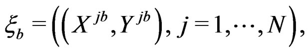
 , where
 . Consider a vector
 .
.
2) Let . Generate bootstrap samples
For each of these samples, construct a CART classifier  and calculate
where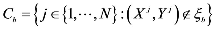 .
.
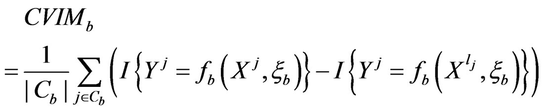
3) Compute the final CVIM using the formula
 . (29)
Any permutation  in the CVIM algorithm destroys dependence between
  and
and  where
where  consists of all components of X which are not in
  At the same time it preserves initial empirical distribution of
  calculated for the sample x. The average loss of correctly classified Y is calculated, and if it is relatively large w.r.t. CVIM of other predictors, then
  plays important role in classification and vice versa.
For instance, as (
( ) one can take all the components
  (
( ) such that the hypothesis of the independence between
  and
and  is not rejected at some significance level (e.g., 5%). CVIM-like algorithm could be used to range combinations of predictors w.r.t. the level of association to the disease. This will be published elsewhere.
3. Applications: Risks of CHD and MI
We employ here various statistical methods described above to analyze the influence of genetic and non-genetic (conventional) factors on risks of coronary heart disease and myocardial infarction using the data for 454 individuals (333 cases, 121 controls) and 333 individuals (165 cases, 168 controls) respectively. These data contain values of seven SNPs and four conventional risk factors. Namely, we consider glycoprotein Ia (GPIa), connexin- 37 (Cx37), plasminogen activator inhibitor type 1 (PAI-1), glycoprotein IIIa (GPIIIa), blood coagulation factor VII (FVII), coagulation factor XIII (FXIII) and interleukin-6 (IL-6) genes, as well as obesity (Ob), arterial hypertension (AH), smoking (Sm) and hypercholesterolemia (HC). The choice of these SNPs was based on biological considerations. For instance, to illustrate this choice we recall that connexin-37 (Cx37) is a protein that forms gapjunction channels between cells. The mechanism of the SNP in Cx37 gene influence on atherosclerosis development is not fully understood, but some clinical data suggest its importance for CHD development [28]. In the Russian population homozygous genotype can induce MI development, especially in individuals without CHD anamnesis [29].
The age of all individuals in case and control groups ranges from 35 to 55 years to reduce its influence on the risk analysis. For each of considered methods, we use K-fold cross-validation with K = 6. As shown in [16], the standard choice of partition number of cross-validation from 6 to 10 does not change the EPE significantly. We take K = 6 as the sample sizes do not exceed 500. The MSU supercomputer “Chebyshev” was involved to perform computations. As shown below, all applied methods permit to choose appropriate models having EPE for CHD dataset less than 0.25. Thus predictions constructed have significant predictive power. Note that, e.g., in [30] the interplay between genotype and MI development was also studied, with estimated prediction errors 0.30 - 0.40.
3.1. MDR and MDRIR Method
Coronary heart disease. Table 1 contains EPEs of the most significant combinations of predictors obtained by MDR analysis of coronary heart disease data. Note that we write the gene meaning the corresponding SNP. To estimate the empirical c.d.f. of the prediction error when the disease is not linked with explanatory variables, we used the permutation test. Namely, 100 random uniform permutations of variables  were generated. For any permutation
  we constructed a sample
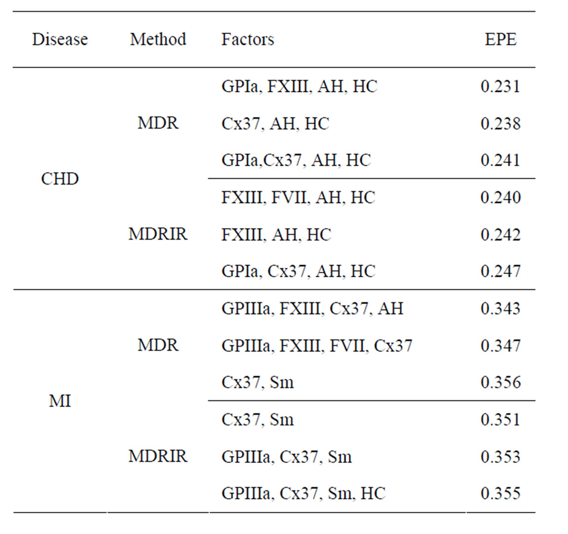
Table 1. The most significant combinations obtained by MDR and MDRIR analysis for CHD and MI data.
and applied the same analysis to this simulated sample, here  In these 100 simulations the corresponding empirical prediction error was not less than 0.42. Thus the Monte Carlo p-value of all three combinations was less than 0.01 (since their EPEs were much less than 0.42), which is usually considered as a good performance.
Table 1 contains also the results of MDRIR method, which are similar to results of MDR method. However, MDRIR method allows to identify additional combinations (listed in this table) with EPE around 0.24. It follows from the same table that hypertension and hypercholesterolemia are the most important non-genetic risk factors. Indeed, these two factors appear in each of 6 combinations.
To perform a more precise analysis of influence of SNPs on CHD provoking we analyzed gene-gene interactions. We used two different strategies. Namely, we applied MDR method to a subgroup of individuals who were not subject to any of the non-genetic risk factors, i.e. to non-smokers without obesity and without hypercholesterolemia, 51 cases and 97 controls (risk-free sample). Another strategy was to apply MDR method to the whole sample, but to take into account only genetic factors rather than all factors. Table 2 contains the most significant combinations of SNPs and their EPEs.
Thus based on coronary heart disease data with the help of Tables 1 and 2 we can make the following conclusions. Combination of two SNPs (in GPIa and Cx37) and two non-genetic factors (hypertension and hypercholesterolemia) has the biggest influence on CHD. Also FXIII gives additional predictive power if AH and HC are taken into account.
It turns out that both methods yield similar results. Combination of SNPs in GPIa and Cx37 has the biggest influence on CHD. EPE is about 0.28 - 0.34, and smaller error corresponds to a risk-free sample. Moreover, it follows from Tables 1 and 2 that EPE dropped significantly after additional non-genetic factors were taken into account (the error is 0.247 if additional non-genetic factors are taken into account and 0.343 if not).
Myocardial infarction. EPEs of the most significant combinations obtained by MDR analysis of MI data are presented in Table 1. For all 100 simulations of  when the disease was not linked with risk factors, EPE was larger than 0.38. Monte Carlo p-value of all combinations was less than 0.01. MDRIR analysis of the same dataset gave a clearer picture (see the same table), as the pair (Cx37, Sm) appears in all three combinations with the least estimated prediction error.
Apparently, combination of smoking and SNP in Cx37 is the most significant. These two factors appear in all combinations in Table 1 concerning MI and MDRIR. Involving any additional factors only increases EPE.
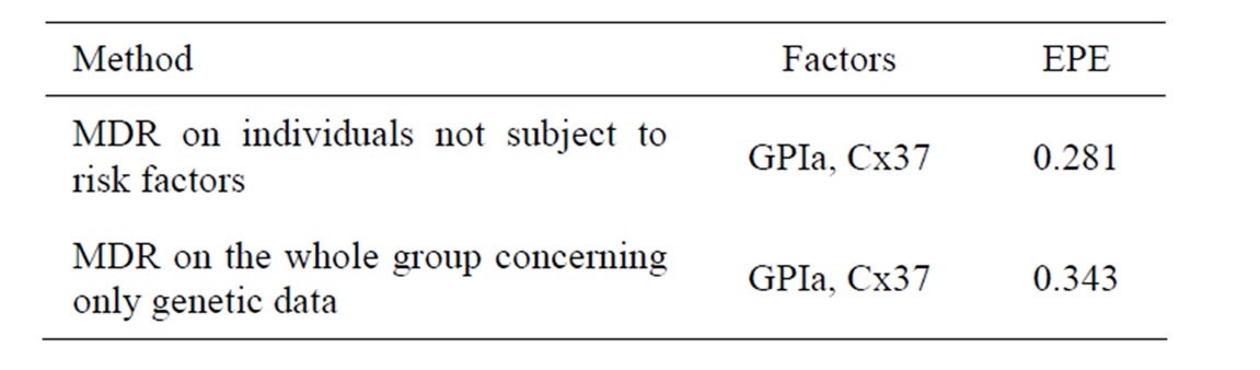
Table 2. Comparison of the most significant SNP combinations obtained by two different ways of MDR analysis of CHD data.
The explicit form of the prediction algorithm based on Cx37 and Sm shows that these factors exhibit interaction. Smoking as well as homozygote for recessive allele of the SNP in Cx37 provokes the disease. However wildtype allele can protect from consequences of smoking. Namely, the combination of smoking and Cx37 wildtype is protective, i.e. the value of prediction algorithm of this combination is –1.
3.2. Ternary Logic Regression
We performed several research procedures for CHD and MI data, with different restrictions imposed on the statistical model. Set
where a vector  stands for SNP values (in PAI‑1, GPIa, GPIIIa, FXIII, FVII, IL-6, Cx37 respectively) and
  denotes non-genetic risk factors (Ob, AH, Sm, HC),
We considered four different models in order to analyze both total influence of genetic and non-genetic factors and losses in predictive force appearing when some factors were excluded. In our applications we took  as search over larger forests for samples with modest sizes could have given very complicated and unreliable results.
Model 1. Define the class M (see Section 2.3) consisting of the functions h having a form

where  and
and  are polynomials identified with trees. In other words we require that non-genetic factors are present only in trees consisting of one variable.
Model 2. Now we assume that any function  has the representation
where  and
and  are polynomials identified with trees. Thus we allow the interaction of genes and nongenetic factors in order to find significant gene-environment interactions. However we impose additional restrictions to avoid too complex combinations of nongenetic risk factors. We do not tackle here effects of interactions where several non-genetic factors are involved. Namely, we consider only the trees satisfying the following two conditions.
1) If there is a leaf containing non-genetic factor variable then the root of that leaf contains product operator.
2) Moreover, another branch growing from the same root is also a leaf and contains a genetic (SNP) variable.
Models 3 and 4 have additional restrictions that polynomials 
 in (30) depend only on nongenetic factors and only on SNPs respectively. These models are considered to compare their results with ones obtained with all information taken into account, in order to demonstrate the importance of genetic (resp. non-genetic) data for risk analysis.
Coronary heart disease. The obtained results are provided in Table 3.
EPE in Model 1 for CHD was only 0.19. For the same model we performed also fast simulated annealing search of the optimal forest which was much more time-efficient, and a reasonable error of 0.23 was obtained. Model 3 application showed that non-genetic factors play an important role in CHD genesis, as classification based on non-genetic factors only gave the error less than 0.23, while usage of SNPs only (Model 4) let the error grow to 0.34.
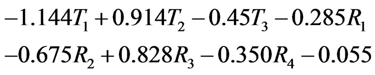
Model 1 gave the minimal EPE. For the optimal forest  the function
  given before formula (28) with
  is provided by
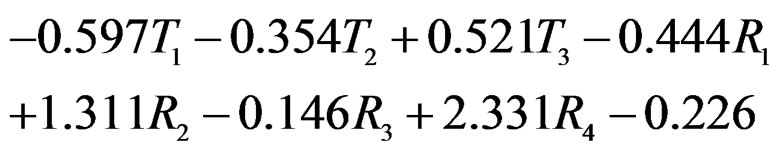 (31)
(31)
where
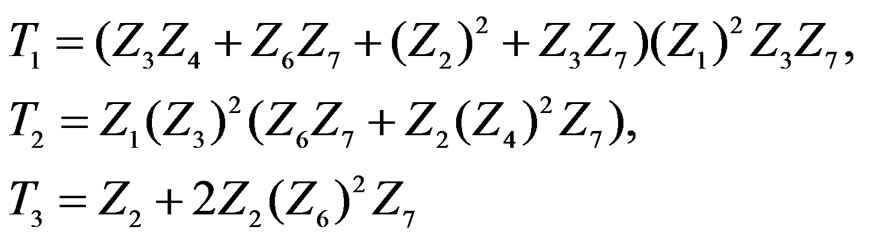
with sums and products modulo 3.
The non-genetic factors 2 and 4 (i.e. AH and HC) are the most influential since the coefficients at them are the greatest ones (1.311 and 2.331). As is shown above, MDR yielded the same conclusion. If the gene-environment interactions were allowed (Model 2), no considerable increase in predictive power has been detected. However we list the pairs of SNPs and non-genetic factors present in the best forest:  and
and ,
,  and
and ,
,  and
and ,
,  and
and  We see that SNP in Cx37 is of substantial importance as it appears in combination with all risk factors except for smoking.
As formula (31) is hard to interpret, we select the most significant SNPs via a variant of permutation test. Consider a random rearrangement of the column with first SNP in CHD dataset. Calculate the EPE using these new simulated data and the same function  as before. The analogous procedure is done for other columns (containing the values of other SNPs) and the errors found are given in Table 4 (recall that the EPE equals 0.19 if no permutation is done).
It is seen that the error increases considerably when the values of GPIa and Cx37 are permuted. The statement that they are the main sources of risk agrees with what was obtained above by MDR method.
Myocardial infarction. For the MI dataset, under the same notation that above, the results obtained for our four models are given in Table 3. To comment them we should first note that non-genetic risk factors play slightly less important role compared with CHD risk: if they are used without genetic information, the error increases by 0.09, see Models 1 and 3 (while the same increase for CHD was 0.03). The function  defined before (28) with
  equals
where .
.
Thus the first tree has the greatest weight (coefficient equals –1.144), the second tree (i.e. SNP in Cx37) is on the second place, and non-genetic factors are less important.
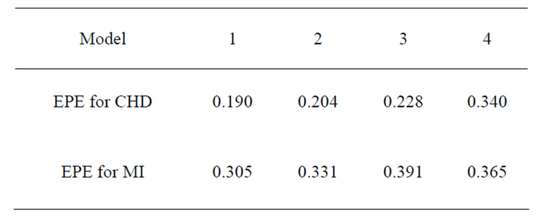
Table 3. Results of TLR.

Table 4. The SNP significance test for CHD in Model 1.
As for CHD we performed a permutation test to compare the significance of different SNPs. Its results are presented in Table 5.
As seen from this table, the elimination of Cx37 SNP leads to a noticeable increase in the EPE. This fact agrees with results obtained by MDR analysis of the same dataset.
3.3. Results Obtained by RF and SGB Methods
Since machine learning methods give too complicated estimates of the dependence structure between Y and X, we have two natural ways to compare them with our methods. Namely, these are the prediction error and the final significance of each predictor. The given datasets were unbalanced w.r.t. response variable and we first applied the resampling technique to them. That means enlargement of the smaller of two groups case-control in the sample by additional bootstrap observations until the final proportion case:control is 1:1. Note that due to the resampling techniques the following effect arises: some observations in small groups (case or control) appear in the new sample more frequently than other ones. Therefore, we took the average over 1000 iterations.
Coronary heart disease. Results of RF and SGB methods are given in Table 6. It shows that RF and SGB methods gave statistically reliable results (EPE in the permutation test is close to 50%). Moreover, additional SNP information improved predicting ability by 13% (SGB). It seems that SGB method is fitted better to CHD data than RF.
To compute CVIM for each , we constructed a vector
  as follows. Let
  contain all predictors
 ,
,  , for which chi-square criteria rejected independence hypothesis between
  and
and  at 5% significance level. Table 7 shows that the most relevant predictors for CHD are AH, HC and Cx37.
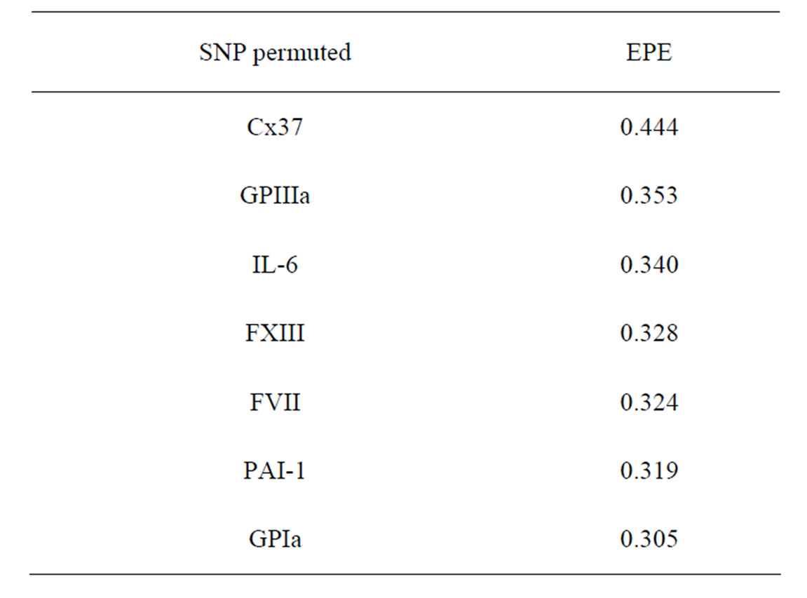
Table 5. The SNP significance test for MI in Model 1.
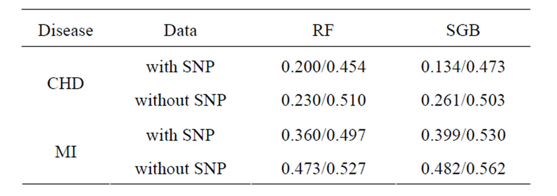
Table 6. EPE/EPE in permutation test calculated via crossvalidation for CHD and MI datasets with employment of RF and SGB methods.
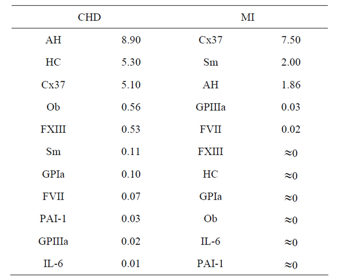
Table 7. Predictors ranged in terms of their CVIM for CHD and MI dataset.
Myocardial infarction. Results of RF and SGB methods are given in Table 6. It shows that RF and SGB methods gave statistically reliable estimates (EPE in the permutation test is close to 50%). Moreover, additional SNP information improved predicting ability by 11% (RF method).
CVIM was calculated according to (29) and is given in Table 7. Thus, the most relevant predictors for MI are Cx37, Sm and AH.
4. Conclusions and Final Remarks
In the current study we developed important statistical methods concerning the analysis of multidimensional genetic data. Namely, we proposed the MDR with independent rule and ternary logic regression with a new version of simulated annealing. We compared them with several popular methods which appeared during the last decade. It is worth to emphasize that all considered methods yielded similar qualitative results for dataset under study.
Let us briefly summarize the main results obtained. The analysis of CHD dataset showed that two non-genetic risk factors out of four considered (AH and HC) had a strong connection with the disease risk (the error of classification based on non-genetic factors only is 0.25 - 0.26 with p-value less than 0.01). Also, the classification based on SNPs only gave an error of 0.28 which is close to one obtained by means of non-genetic predictors. Moreover, the most influential SNPs were in genes Cx37 and GPIa (FXIII also entered the analysis only when AH and HC were present). EPE decreased to 0.13 when both SNP information and non-genetic risk factors were taken into account and SGB was employed. Note that excludeing any of the 5 remaining SNPs (all except for two most influential) from data increased the error by 0.01 - 0.02 approximately. So, while the most influential data were responsible for the situation within a large part of population, there were smaller parts where other SNPs came to effect and provided a more efficient prognosis (“small subgroups effect”). The significance of SNP in GPIa and FXIII genes was observed in our work. AH and HC influence the disease risk by affecting the vascular wall, while GPIa and FXIII may improve prognosis accuracy because they introduce haemostatic aspect into analysis.
The MI dataset gave the following results. The most significant factors of MI risk were the SNP in Cx37 (more precisely, homozygous for recessive allele) and smoking with a considerable gene-environment interacttion present. The smallest EPE of methods applied was 0.33 - 0.35 (with p-value less than 0.01). The classification based on non-genetic factors only yielded a greater error of 0.42. Thus genetic data improved the prognosis quality noticeably. While two factors were important, other SNPs considered actually did not improve the prognosis essentially, i.e. no small groups effect was observed.
While CHD data used in the study permitted to specify the most important predictors with EPE about 0.13, the MI data lead to less exact prognoses. Perhaps this complex disease requires a more detailed description of individual’s genetic characteristics and environmental factors.
The conclusions given above are based on several complementary methods of modern statistical analysis. These new data mining methods allow to analyze other datasets as well. The study can be continued and the medical conclusions need to be replicated with larger datasets, in particular, involving new SNP data.
5. Acknowledgements
The work is partially supported by RFBR grant (project 10-01-00397a).
REFERENCES
- Y. Fujikoshi, R. Shimizu and V. V. Ulyanov, “Multivariate Statistics: High-Dimensional and Large-Sample Approximations,” Wiley, Hoboken, 2010.
- S. Szymczak, J. Biernacka, H. Cordell, O. GonzálezRecio, I. König, H. Zhang and Y. Sun, “Machine Learning in Genome-Wide Association Studies,” Genetic Epidemiology, Vol. 33, No. S1, 2009, pp. 51-57. doi:10.1002/gepi.20473
- D. Brinza, M. Schultz, G. Tesler and V. Bafna, “RAPID Detection of Gene-Gene Interaction in Genome-Wide Association Studies”, Bioinformatics, Vol. 26, No. 22, 2010, pp. 2856-2862. doi:10.1093/bioinformatics/btq529
- K. Wang, S. P. Dickson, C. A. Stolle, I. D. Krantz, D. B. Goldstein and H. Hakonarson, “Interpretation of Association Signals and Identification of Causal Variants from Genome-Wide Association Studies,” The American Journal of Human Genetics, Vol. 86, No. 5, 2010, pp. 730-742. doi:10.1016/j.ajhg.2010.04.003
- Y. Liang and A. Kelemen. “Statistical Advances and Challenges for Analyzing Correlated High Dimensional SNP Data in Genomic Study for Complex Diseases,” Statistics Surveys, Vol. 2, No. 1, 2008, pp. 43-60. doi:10.1214/07-SS026
- H. Schwender and I. Ruczinski, “Testing SNPs and Sets of SNPs for Importance in Association Studies,” Biostatistics, Vol. 12, No. 1, 2011, pp. 18-32. doi:10.1093/biostatistics/kxq042
- M. Ritchie, L. Hahn, N. Roodi, R. Bailey, W. Dupont, F. Parl and J. Moore, “Multifactor-Dimensionality Reduction Reveals High-Order Interactions among EstrogenMetabolism Genes in Sporadic Breast Cancer,” The American Journal of Human Genetics, Vol. 69, No. 1, 2001, pp. 138-147. doi:10.1086/321276
- D. Velez, B. White, A. Motsinger, W. Bush, M. Ritchie, S. Williams and J. Moore, “A Balanced Accuracy Function for Epistasis Modeling in Imbalanced Datasets Using Multifactor Dimensionality Reduction,” Genetic Epidemiology, Vol. 31, No. 4, 2007, pp. 306-315. doi:10.1002/gepi.20211
- I. Ruczinski, C. Kooperberg and M. LeBlanc, “Logic Regression,” Journal of Computational and Graphical Statiststics, Vol. 12, No. 3, 2003, pp. 475-511. doi:10.1198/1061860032238
- H. Schwender and K. Ickstadt, “Identification of SNP Interactions Using Logic Regression,” Biostatistics, Vol. 9, No. 1, 2008, pp. 187-198. doi:10.1093/biostatistics/kxm024
- L. Breiman, “Random Forests,” Machine Learning, Vol. 45, No. 1, 2001, pp. 5-32. doi:10.1023/A:1010933404324
- J. Friedman, “Stochastic Gradient Boosting,” Computational Statistics & Data analysis, Vol. 38, No. 4, 2002, pp. 367-378. doi:10.1016/S0167-9473(01)00065-2
- X. Wan, C. Yang, Q. Yang, H. Xue, N. Tang and W. Yu, “Mega SNP Hunter: A Learning Approach to Detect Disease Predisposition SNPs and High Level Interactions in Genome Wide Association Study,” BMC Bioinformatics, Vol. 10, 2009, p. 13. doi:10.1186/1471-2105-10-13
- A. Bulinski, O. Butkovsky, A. Shashkin, P. Yaskov, M. Atroshchenko and A. Khaplanov, “Statistical Methods of SNPs Analysis,” Technical Report, 2010, pp. 1-159 (in Russian).
- G. Bradley-Smith, S. Hope, H. V. Firth and J. A. Hurst, “Oxford Handbook of Genetics,” Oxford University Press, New York, 2010.
- S. Winham, A. Slater and A. Motsinger-Reif, “A Comparison of Internal Validation Techniques for Multifactor Dimensionality Reduction,” BMC Bioinformatics, Vol. 11, 2010, p. 394. doi:10.1186/1471-2105-11-394
- A. Arlot and A. Celisse, “A Survey of Cross-Validation Procedures for Model Selection,” Statistics Surveys, Vol. 4, No. 1, 2010, pp. 40-79. doi:10.1214/09-SS054
- T. Hastie, R. Tibshirani and J. Friedman, “The Elements of Statistical Learning: Data Mining, Inference, and Prediction,” 2nd Edition, Springer, New York, 2009.
- R. L. Taylor and T.-C. Hu, “Strong Laws of Large Numbers for Arrays of Rowwise Independent Random Elements,” International Journal of Mathematics and Mathematical Sciences, Vol. 10, No. 4, 1987, pp. 805-814. doi:10.1155/S0161171287000899
- E. Lehmann and J. Romano, “Testing Statistical Hypotheses,” Springer, New York, 2005.
- P. Golland, F. Liang, S. Mukherjee and D. Panchenko, “Permutation Tests for Classification,” Lecture Notes in Computer Science, Vol. 3559, 2005, pp. 501-515. doi:10.1007/11503415_34
- J. Park, “Independent Rule in Classification of Multivariate Binary Data,” Journal of Multivariate Analysis, Vol. 100, No. 10, 2009, pp. 2270-2286. doi:10.1016/j.jmva.2009.05.004
- S. Lee, Y. Chung, R. Elston, Y. Kim and T. Park, “LogLinear Model-Based Multifactor Dimensionality Reduction Method to Detect Gene-gene Interactions,” Bioinformatics, Vol. 23, No. 19, 2007, pp. 2589-2595. doi:10.1093/bioinformatics/btm396
- A. Nikolaev and S. Jacobson, “Simulated Annealing,” In: M. Gendreau and J.-Y. Potvin, Eds., Handbook of Metaheuristics, Springer, New York, 2010, pp. 1-39.
- G. Biau, “Analysis of a Random Forests Model,” LSTA, LPMA, Paris, 2010.
- N. Chawla, “Data Mining for Imbalanced Datasets: An Overview,” In: O. Maimon and L. Rokach, Eds., Data Mining and Knowledge Discovery Handbook, Springer, New York, 2010, pp. 875-886.
- C. Strobl, A. Boulesteix, T. Kneib, T. Augustin and A. Zeileis, “Conditional Variable Importance for Random Forests,” BMC Bioinformatics, Vol. 9, 2008, p. 307. doi:10.1186/1471-2105-9-307
- A. Hirashiki, Y. Yamada, Y. Murase, Y. Suzuki, H. Kataoka, Y. Morimoto, T. Tajika, T. Murohara and M. Yokota, “Association of Gene Polymorphisms with Coronary Artery Disease in Lowor High-Risk Subjects Defined by Conventional Risk Factors,” Journal of the American College of Cardiology, Vol. 42, No. 8, 2003, pp. 1429-1437. doi:10.1016/S0735-1097(03)01062-3
- A. Balatskiy, E. Andreenko and L. Samokhodskaya, “The Connexin37 Polymorphism as a New Risk Factor of MI Development,” Siberian Medical Journal, Vol. 25, No. 2, 2010, pp. 64-65 (in Russian).
- C. Coffey, P. Hebert, M. Ritchie, H. Krumholz, J. Gaziano, P. Ridker, N. Brown, D. Vaughan and J. Moore, “An Application of Conditional Logistic Regression and Multifactor Dimensionality Reduction for Detecting GeneGene Interactions on Risk of Myocardial Infarction: The Importance of Model Validation,” BMC Bioinformatics, Vol. 5, 2004, p. 49. doi:10.1186/1471-2105-5-49
NOTES
*Corresponding author.