American Journal of Operations Research
Vol.06 No.01(2016), Article ID:63034,10 pages
10.4236/ajor.2016.61008
A Production Inventory Model of Constant Production Rate and Demand of Level Dependent Linear Trend
Shirajul Islam Ukil, Md. Sharif Uddin
Jahangirnagar University, Savar, Bangladesh

Copyright © 2016 by authors and Scientific Research Publishing Inc.
This work is licensed under the Creative Commons Attribution International License (CC BY).
http://creativecommons.org/licenses/by/4.0/


Received 2 December 2015; accepted 22 January 2016; published 26 January 2016
ABSTRACT
The proposed model considers the products with finite shelf-life which causes a small amount of decay. The market demand is assumed to be level dependent and in a linear form. The model has also considered the constant production rate which stops attaining a desired level of inventories and that is the highest level of inventories. Production starts with a buffer stock and without any sort of backlogs. Due to the market demand and product’s decay, the inventory reduces to the level of buffer stock where again the production cycle starts. With a numerical search procedure the proof of the proposed model has been shown. The objective of the model is to obtain the total average optimum inventory cost and optimum ordering cycle.
Keywords:
Production Inventory, Level Dependent Linear Trend, Constant Production Rate

1. Introduction
With a view to solving the inventory problems, it is highly essential for the business institutions to obtain the economic order quantity (EOQ) and obtaining this quantity leads to reduce the total average inventory cost. This is why the business institutions emphasize on inventory management and solving inventory problems. The problem can only be solved if a suitable inventory model could be established which is fit for all the parameters concerned like, market demand, production rate, product’s life, etc. The innovative EOQ model is, therefore, a highly demand on regular basis and when required in spite of having existence of huge number of inventory models. Inventory, indeed, is a stock of materials. Inventory problems are mainly related to the proper management of this inventory which can lead to minimize the inventory cost. Generally, we have two kinds of materials in our daily needs as far as damage, wastage, deterioration or decay is concerned. Items like radioactive substances, food grains, fashionable items, pharmaceuticals, etc. are the items of finite life and the items like electronic goods, steels, woods, etc. are the items of ling life. Due to the limited shelf-life and market demand, the stock level or inventory continuously decreases and the items in the inventory deplete or deteriorate. This deterioration affects the inventory and inventory cost increases. To make the inventory cost at optimum level i.e. to get the minimum inventory cost, a suitable inventory model is required to be formulated. An inventory model with linear demand, small amount of decay and constant production rate has been proposed in this paper to minimize inventory cost. Keeping the buffer stock as a reserve, the production is assumed to start and after certain periods at the highest level of inventory, it stops. In this model, we have considered constant production rate along with the deterioration, whereas the classical inventory models and many researchers use the instantaneous replenishment. Finally, by proving the convex property and using a numerical searcher procedure, the paper justified the correctness of the model.
2. Literature Review
Since long the researchers had been focusing on obtaining inventory models suitable to the needs in real life with a view to solving inventory problems. The problems are related with what will be the pattern of demand in the market, what may be the production rate of the business institutions, whether there will be finite life of the products, whether backlogs or shortages and delay in payments are allowed etc. Many researchers have structured various types of inventory model basing on the situation or the market demand. It may arise different types of demands in the market. Demand may be linear, quadratic, exponential, time dependent, level or stock dependent, price dependent etc. Considering all the parameters the inventory model is designed. There are two types of models in this field which covers all the parameters mentioned above. One is deterministic model which deals with the constant demand and lead time; the other one is stochastic or probabilistic model which deals randomly with the variable demand and lead time. In this review of the literature, mostly the inventory models with deterministic demand have been discussed. Determining EOQ is one of the most important factors to formulate the inventory model. The ultimate aim of formulating the model is to minimize the inventory cost by finding the EOQ. Harris [1] was the first researcher to study the inventory model. The new horizon is opened in the field of the inventory control management since he presented the famous EOQ formula. Whitin [2] developed the inventory model for the first time which was suitable for fashionable goods considering its little decay in the inventory. Ghare and Schrader [3] first pointed out the effect of decay in inventory analysis and discovered the economic order quantity (EOQ) model. They showed the nature of the consumption of the deteriorating items. Skouri and Papachristos [4] discussed a continuous review inventory model considering the five costs as deterioration, holding, shortage, opportunity cost due to the lost sales and the replenishment cost due to the linearly dependency on the lot size. Chund and Wee [5] developed an integrated two stages production inventory deteriorating model for the buyer and the supplier on the basis of stock dependent selling rate considering imperfect items and just in time (JIT) multiple deliveries. Applying inventory replenishment policy Cheng and Wang [6] expressed the inventory model for deteriorating items with trapezoidal type demand rate, where the demand rate is a piecewise linearly functions. Hassan and Bozorgi [7] developed the location of distribution centers with inventory. Sarker et al. [8] explained an inventory model where demand was a composite function consisting of a constant component and a variable component proportional to inventory level in a period in which decay was exponential and inventory was positive. Tripathy and Mishra [9] discuss the inventory model with ordering policy for weibull deteriorating items, quadratic demand, and permissible delay in payments. Khieng et al. [10] presented a production model for the lot-size, order level inventory system with finite production rate and the effect of decay. Ekramol [11] [12] considered various production rates assuming the demand is constant. Mishra et al. [13] explained an inventory model for deteriorating items with time dependent demand and time varying holding cost under partial backlogging. Ukil [14] discussed the effect of just in time manufacturing system on EOQ model. Sivazlian and Stenfel [15] determined the optimum value of time cycle by using the graphical solution of the equation to obtain the economic order quantity model. Shah and Jaiswal [16] and Dye [17] established an inventory model by considering demand as a function of selling price and three parameters of Weibull rate of deterioration. Billington [18] discussed classic economic production quantity (EPQ) model without backorders or backlogs. Pakkala and Achary [19] established a deterministic inventory model for deteriorating items with two warehouses, while the replenishment rate was finite, demand was uniform and shortage was allowed. Abad [20] discussed regarding optimal pricing and lot sizing under conditions of perish ability and partial backordering. Sing and Pattanak [21] - [23] developed the model for deterioration and time dependent quadratic demand under permissible delay in payment, whereas we have used the demand of linear trend but ignoring the payment aspect. Amutha and Chandrasekaran [24] formulated the inventory model with deterioration items, quadratic demand and time dependent holding cost, but in our proposed model, we have emphasized on the production rate, linear type of demand and constant holding cost. Ouyang and Cheng [25] explained the inventory model for deteriorating items with exponential declining demand and partial backlogging. Dave and Patel [26] introduced an inventory model for deteriorating Items with time proportional demand, but we have considered the demand which is level dependent and a type of linear trend. Teng et al. [27] developed the model with deteriorating items and shortages assuming that the demand function was positive and fluctuating with respect to time, but in the proposed model, the demand was considered as a linear function and production starts with a buffer stock as a reserve. The previous model established various types of inventory models considering several parameters which did not consider the production rate, linear demand along with the buffer stock. Here comes the necessity to build the proposed model.
3. Assumptions and Notations
・ Production rate  is constant and greater than demand rate at any time.
・  = Demand rate at any instant
 , where “
 ” and
” and  satisfying the condition
 .
.
・ For unit inventory, amount of decay rate  is very small and constant.
・ Production starts with a few amounts of items in the inventory as a buffer stock.
・ Inventory level is highest at a specific level and after this point, the inventory depletes quickly due to demand and deterioration.
・ Shortages are not allowed.
・  = Inventory level at instant
 .
.
・  = Un-decayed inventory at
  to
to .
.
・  = Un-decayed inventory at
  to
to .
.
・  = Deteriorating inventory at
  to
to .
.
・  = Deteriorating inventory at
  to
to .
.
・  and Q = Inventory level at time
 ,
,  and
and  respectively. Here, Q is the buffer stock.
・  = Vary small portion of instant
 .
.
・  = Set up cost.
・  = Average holding cost.
・  = Total average inventory cost in terms of
 .
.
・  = Time when inventory gets maximum level.
・  = Total time cycle.
・  = Optimum order quantity.
・  = Optimum time at maximum inventory.
・  = Optimum order interval.
・  = Total average optimum inventory cost.
4. Formulation of the Model
Basing on the demand pattern, the business institution decides the structure of the model (Figure 1). This demand very often changes because of various reasons. In reality, the demand may at times the demand be dependent on the level or the stock on hand in the inventory. To meet this type of situation, this model is developed. The model is suitable for those kinds of products which have finite shelf-life and ultimately causes the products decay due to its limited life. At the beginning, while time , the production
  starts with Q inventories and the production remains constant for entire production cycle.
The inventory increases at the rate of 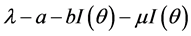 during
  to
to . The market demand is
 and
and  is the decay of
  inventories at instant
  where,
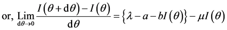
  is the decay of unit inventory in the mentioned period. With the help of the above criteria we can formulate the differential equations as

Figure 1. Inventory model with linear demand.
below:


The general solution of the differential equation is .
.
Applying the following boundary condition, we get  at
at , Solving these equations, we get,
 ,
,
Therefore,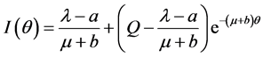 (1)
(1)
From the other boundary condition, i.e. at ,
,  , taking up to first degree of
 , we get the following equation:
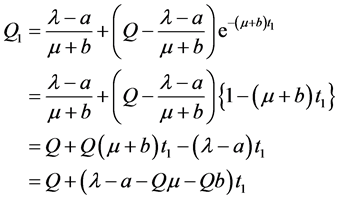 (2)
(2)
Using the Equation (1) and considering up to second degree of  for our convenience, the total undecayed inventory during
  to
to  we get,
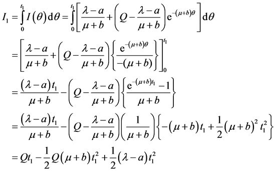 (3)
(3)
We calculate the deteriorating items during the period considering the decay of the items as below:
 (4)
(4)
On the other hand, the inventory decreases at the rate of  during
  to
to  as there is no production after time
 . The inventory depletes due to market demand and the deterioration of the items. Similar approach as used before can be applied to get another differential equation which is as follows:

The general solution of the differential equation is defined below:

Applying the boundary condition at , we get,
 .
.
By solving we get, .
.
Therefore, (5)
(5)
Substituting another boundary condition, i.e. at ,
,  , taking up to first order of
 , we get the following equation:
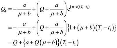 (6)
(6)
Now, using Equation (5) and considering up to the first degree of  we get the un-decayed inventory during
  to
to  as:
as:
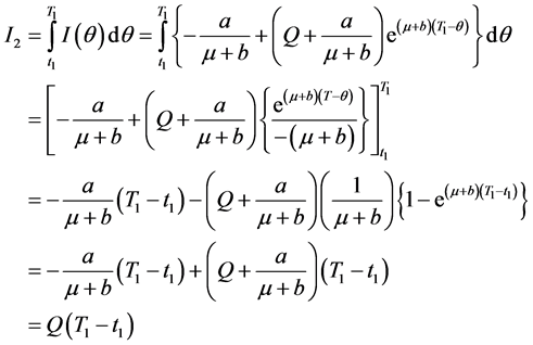 (7)
(7)
Considering the decay of the items, we calculate the deteriorating items during the period as below:
 (8)
(8)
From Equations (2) and (6), we get,

Or,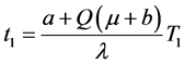 (9)
(9)
Considering the value as  (10)
(10)
We construct the following equation with the help of Equation (9),
 (11)
(11)
Total Cost Function: The cost function can be described in the following form,
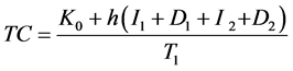 (12)
(12)
By substituting the Equations (3), (4), (7), (8) and (11) in (12), we get the value of total average inventory cost as below,
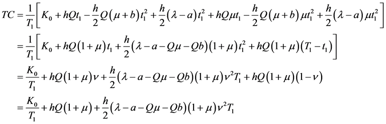 (13)
(13)
Now with a view to obtaining the total time cycle  that minimizes the total average inventory cost for the inventory system we shall adopt the convex property. The total average inventory cost is depicted by the equation no (13). To obtain the optimum time cycle and verify Equation (13) as convex in
 , we must satisfy the following well established convex property,
(i)  and
and
(ii) 
Now differentiating Equation (13) with respect to  we get the following equation,
 (14)
(14)
Putting the value of Equation (14) in the convex property (i) and then using (10), we get

Or, 
Or, (15)
(15)
Now with the help of Equations (11) and (15), we get the value of  as below,
 (16)
(16)
Again differentiating Equation (14) with respect to , we get,
 (17)
(17)
From Equation (17) we come to an end that the convex property (ii) is satisfied, i.e. , as
, as  and
and
 both is positive. Finally, we conclude that total cost function (13) is convex in
 . Hence, there is an optimal solution in
  for which the total average inventory cost must be minimal.
5. Numerical Search Procedure
According to the result in section 5, we give an example that may illustrate how the numerical search procedure works. Suppose that there is a product which is a linear function in the inventory system and adopts the following parameters:

We now put all the values in Equations (15), (16), (2) and (13) and then we get the results as optimum order interval  units, optimum time
  units at maximum inventory level, optimum order quantity
 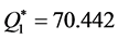 units and total average optimum inventory cost
  units respectively. Substituting the values of
  arbitrarily either bigger or lesser than
 , we get the inventory cost gradually increased from the minimum inventory cost at optimum level, which is show in Table 1 and Figure 2. The table and figure justify the total average optimum inventory cost. If we analyze the table and figures we can observe that in a particular point total inventory cost is minimal and the order interval is optimum.
6. Sensitivity Test
Now, how the inventory system or the solution is affected by even a little changes of parameters  and
and

Table 1. Order interval ( ) verses total cost (
 ).
).
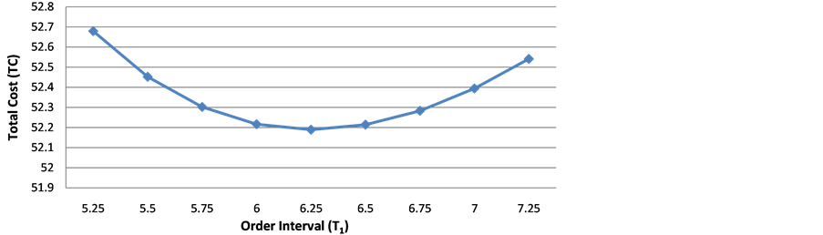
Figure 2. Time verses total cost.
Table 2. Effects of the changes of parameters.
 on the optimal time
  at maximum inventory level, optimum length of ordering cycle
 , optimal order quantity
  and the total average optimum inventory cost
  per unit time in the model, will be shown in the following table. If the parameters change the values mentioned in Table 2 by adding and subtracting respectively, we see the effect on the on the optimal time
  at maximum inventory level, optimum length of ordering cycle
 , optimal order quantity
  and the total average optimum inventory cost
  per unit time. While the change of one parameter take place, the other parameter must remain unchanged. Table 2 shows the effect or the sensitivity.
Table 2 shows that small amount of a particular parameter may affect on the values of  and
and  even on great extent. On the basis of the results obtained in Table 2, the following observations can be highlighted:
・  and
and  decrease while
  and
and  increase with increase in the value of the parameter
 . Here
  is highly sensitive to
  and moderately sensitive to other values.
・  and
and  increase while
  and
and  decrease with increase in the value of the parameter
  and b. Here,
  and
and  all are moderately sensitive to the values of
  and
and .
.
・  and
and  decrease, while
  increases with increase in the value of the parameter
 . Here,
  is moderately sensitive to all the values of
  and
and .
.
・  and
and  decrease and
  increases, while
  remain unchanged with increase in the value of the parameter h. Here, h is highly sensitive to the value of
  and moderately sensitive to all other values.
7. Conclusion
Because of the development of inventory management in the present age, the business institution cannot think its cost minimization without the proper use of it. By the proper use, management and thereby developing the suitable inventory models, the business enterprise can save its huge inventory cost. Before using model the enterprise needs to know the actual pattern of demand in the market. This demand always fluctuates. The suitable model is developed by considering the actual demand. The inventory model we have proposed in this paper is dependent on the stock, even we have considered buffer stock. Hence, the stock goes out due to any unavoidable circumstances, demand could still be met. The model also considers the deterioration, so due to the finite shelf-life of the items this model gives the correct. In the proposed model, the production rate and the decay have been considered constant through. The model develops an algorithm to determine the optimum ordering cost, total average optimum inventory cost, optimum time at maximum inventory level and optimum time cycle. The model could establish that with a particular order level , the total average optimum inventory cost
  units.
Acknowledgements
The authors thank the editor and the reviewers for their valuable comments which could play a significant role to improve the standard of the manuscript.
Cite this paper
ShirajulIslam Ukil,Md. SharifUddin, (2016) A Production Inventory Model of Constant Production Rate and Demand of Level Dependent Linear Trend. American Journal of Operations Research,06,61-70. doi: 10.4236/ajor.2016.61008
References
- 1. Harris, F.W. (1957) Operations and Costs. A. W. Shaw Company, Chicago, 48-54.
- 2. Whitin, T.M. (1957) Theory of Inventory Management. Princeton University Press, Princeton, NJ, 62-72.
- 3. Ghare, P.M. and Schrader, G.F. (1963) A Model for an Exponential Decaying Inventory. Journal of Industrial Engineering, 14, 238-243.
- 4. Skouri, K. and Papachristos, S. (2002) A Continuous Review Inventory Model, with Deteriorating Items, Time Varying Demand, Linear Replenishment Cost, Partially Time Varying Backlogging. Applied Mathematical Modeling, 26, 603-617.
http://dx.doi.org/10.1016/S0307-904X(01)00071-3 - 5. Chund, C.J. and Wee, H.M. (2008) Scheduling and Replenishment Plan for an Integrated Deteriorating Inventory Model with Stock-Dependent Selling Rate. International Journal of Advanced Manufacturing Technology, 35, 665-679.
http://dx.doi.org/10.1007/s00170-006-0744-7 - 6. Cheng, M.B. and Wang, G.Q. (2009) A Note on the Inventory Model for Deteriorating Items with Trapezoidal Type Demand Rate. Computers and Industrial Engineering, 56, 1296-1300.
http://dx.doi.org/10.1016/j.cie.2008.07.020 - 7. Shavandi, H. and Sozorgi, B. (2012) Developing a Location Inventory Model under Fuzzy Environment. International Journal of Advanced Manufacturing Technology, 63, 191-200.
http://dx.doi.org/10.1007/s00170-012-3897-6 - 8. Sarker, B.R. Mukhaerjee, S. and Balam, C.V. (1997) An Order-Level Lot Size Inventory Model with Inventory-Level Dependent Demand and Deterioration. International Journal of Production Economics, 48, 227-236.
http://dx.doi.org/10.1016/S0925-5273(96)00107-7 - 9. Tripathy, C.K. and Mishra, U. (2010) Ordering Policy for Weibull Deteriorating Items for Quadratic Demand with Permissible Delay in Payments. Applied Mathematical Science, 4, 2181-2191.
- 10. Khieng, J.H., Labban. J. and Richard, J.L. (1991) An Order Level Lot Size Inventory Model for Deteriorating Items with Finite Replenishment Rate. Computers Industrial Engineering, 20, 187-197.
http://dx.doi.org/10.1016/0360-8352(91)90024-Z - 11. Ekramol, I.M. (2004) A Production Inventory Model for Deteriorating Items with Various Production Rates and Constant Demand. Proceedings of the Annual Conference of KMA and National Seminar on Fuzzy Mathematics and Applications, Payyanur, 8-10 January 2004, 14-23.
- 12. Ekramol, I.M. (2007) A Production Inventory with Three Production Rates and Constant Demands. Bangladesh Islamic University Journal, 1, 14-20.
- 13. Mishra, V.K., Singh, L.S. and Kumar, R. (2013) An Inventory Model for Deteriorating Items with Time Dependent Demand and Time Varying Holding Cost under Partial Backlogging. Journal of Industrial Engineering International, 9, 1-4.
http://dx.doi.org/10.1186/2251-712x-9-4 - 14. Ukil, S.I., Ahmed, M.M., Sultana, S. and Sharif, U.M. (2015) Effect on Probabilistic Continuous EOQ Review Model after Applying Third Party Logistics. Journal of Mechanics of Continua and Mathematical Science, 9, 1385-1396.
- 15. Sivazlin, B.D. and Stenfel, L.E. (1975) Analysis of System in Operations Research. 203-230.
- 16. Shah, Y.K. and Jaiswal, M.C. (1977) Order Level Inventory Model for a System of Constant Rate of Deterioration. Opsearch, 14, 174-184.
- 17. Dye, C.Y. (1915) Joint Pricing and Ordering Policy for a Deteriorating Inventory with Partial Backlogging. Omega, 35, 184-189.
http://dx.doi.org/10.1016/j.omega.2005.05.002 - 18. Billington, P.L. (1987) The Classic Economic Production Quantity Model with Set up Cost as a Function of Capital Expenditure. Decision Series, 18, 25-42.
http://dx.doi.org/10.1111/j.1540-5915.1987.tb01501.x - 19. Pakkala, T.P.M. and Achary, K.K. (1992) A Deterministic Inventory Model for Deteriorating Items with Two Warehouses and Finite Replenishment Rate. European Journal of Operational Research, 57, 71-76.
http://dx.doi.org/10.1016/0377-2217(92)90306-T - 20. Abad, P.L. (1996) Optimal Pricing and Lot Sizing under Conditions of Perish Ability and Partial Backordering. Management Science, 42, 1093-1104. http://dx.doi.org/10.1287/mnsc.42.8.1093
- 21. Singh, T. and Pattnayak, H. (2013) An EOQ Model for Deteriorating Items with Linear Demand, Variable Deterioration and Partial Backlogging. Journal of Service Science and Management, 6, 186-190.
http://dx.doi.org/10.4236/jssm.2013.62019 - 22. Singh, T. and Pattnayak, H. (2012) An EOQ Model for a Deteriorating Item with Time Dependent Exponentially Declining Demand under Permissible Delay in Payment. IOSR Journal of Mathematics, 2, 30-37.
http://dx.doi.org/10.9790/5728-0223037 - 23. Singh, T. and Pattnayak, H. (2013) An EOQ Model for a Deteriorating Item with Time Dependent Quadratic Demand and Variable Deterioration under Permissible Delay in Payment. Applied Mathematical Science, 7, 2939-2951.
- 24. Amutha, R. and Chandrasekaran, E. (2013) An EOQ Model for Deteriorating Items with Quadratic Demand and Tie Dependent Holding Cost. International Journal of Emerging Science and Engineering, 1, 5-6.
- 25. Ouyang, W. and Cheng, X. (2005) An Inventory Model for Deteriorating Items with Exponential Declining Demand and Partial Backlogging. Yugoslav Journal of Operation Research, 15, 277-288.
http://dx.doi.org/10.2298/YJOR0502277O - 26. Dave, U. and Patel, L.K. (1981) (T, Si) Policy Inventory Model for Deteriorating Items with Time Proportional Demand. Journal of the Operational Research Society, 32, 137-142.
- 27. Teng, J.T., Chern, M.S. and Yang, H.L. (1999) Deterministic Lot Size Inventory Models with Shortages and Deteriorating for Fluctuating Demand. Operation Research Letters, 24, 65-72.
http://dx.doi.org/10.1016/S0167-6377(98)00042-X