American Journal of Operations Research Vol.05 No.03(2015), Article
ID:56610,9 pages
10.4236/ajor.2015.53016
An Alternative Approach to the Lottery Method in Utility Theory for Game Theory
William P. Fox
Department of Defense Analysis, Naval Postgraduate School, Monterey, USA
Email: wpfox@nps.edu
Copyright © 2015 by author and Scientific Research Publishing Inc.
This work is licensed under the Creative Commons Attribution International License (CC BY).
http://creativecommons.org/licenses/by/4.0/


Received 11 March 2015; accepted 22 May 2015; published 25 May 2015
ABSTRACT
In game theory, in order to properly use mixed strategies, equalizing strategies or the Nash arbitration method, we require cardinal payoffs. We present an alternative method to the possible tedious lottery method of von Neumann and Morgenstern to change ordinal values into cardinal values using the analytical hierarchy process. We suggest using Saaty’s pairwise comparison with combined strategies as criteria for players involved in a repetitive game. We present and illustrate a methodology for moving from ordinal payoffs to cardinal payoffs. We summarize the impact on how the solutions are achieved.
Keywords:
Analytical Hierarchy Process, Cardinal Utility, Game Theory, Payoff Matrix

1. Introduction
We teach a three-course sequence in mathematical modeling at the Naval Postgraduate School. In our final course, Models of Conflict, we present an introduction to the following topics: decision theory, multi-attribute decision making with the analytical hierarchy process (AHP) and technique of order preference by similarity to ideal solution (TOPSIS), and game theory.
In game theory, we spend about two lessons on utility theory including the lottery method by von Neumann and Morgenstern. Our students find the back & forth lottery method tedious and they usually do not feel they have the true expertise to narrow in on a true lottery preference. We are currently using Straffin’s chapter 9 for utility theory [1] .
For years, our student’s projects and research in two-person non-zero sum games have used ordinal payoffs. They feel comfortable prioritizing the outcomes in an ordinal manner. They can rank first to last place. If no pure strategies solutions existed, the students assumed that the ordinal payoffs were cardinal payoffs to illustrate the methodologies to obtain equilibrium with mixed strategy solutions.
To add more realism to these projects and eventual research, we present a method to obtain cardinal payoffs that is not tedious and follows from material we have already presented in class using multi-attribute decision making, AHP. In this paper, we describe the issue more fully and describe our methodology using AHP. We provide an example illustrating the technique.
2. Ordinal versus Cardinal Utility
Ordinal utility is a method that ranks outcomes. We tell our students it is like knowing the names of how people finish in a race, 1st, 2nd, 3rd, …, last. Cardinal utility uses interval scale values where we would now replace the order of finish with the times they ran the race. With the times, we know how much faster each runner is compared to the other runners.
Often real data is not available for analysis in a game theory scenario. Perhaps the best students can initially do is “rank order” the outcomes from 1 to n for each player in the game.
3. Lottery Method Illustrated
Consider an example where we have a choice between going to McDonald’s or going to Burger King. Assume that we limit ourselves to the following meal choices:
Burger King: Whopper &French Fries Combo (x), Whopper Jr. &French Fries Combo (y).
McDonalds: Big Mac & French Fries Combo (w), Quarter pounder &French Fries Combo (z).
Step 1. We need an ordinal preference of these choices. Let’s assume the row preferences are:
z > x > y> w.
Step 2. Use the lottery method to assign values: start by assigning z and w arbitrarily keeping in mind that z gets a higher value than w. We could use a scale from [0, 100] and assign 100 to Z and 0 to W, as an example.
Step 3. Next, consider x. Would you prefer x for certain or a lottery which gives you z at 50% of the time and w at 50% of the time. ½ z ½ w? If Rose likes x over the lottery then x ranks higher than the midpoint between z and w. So we use number greater than 50. So you try, would you prefer x for certain or a lottery that gives ¼ w ¾ z? Now, if Rose prefers the lottery then x has value between 50 and 75. We continue until we narrow the value to a point. When Rose is indifferent between the certainty and the lottery we are done. Assume this occurs at 40% w and 60% z. We then would take 60% of 100 for the value of x.
Step 4. We do the same thing for y. Assume, we go through our process and we assign a value of 20 for y.
Step 5. Now, become the column player.
Step 6-Step 9. Repeat step 1 - 4 to obtain values for the column player’s preferences.
This could eventually lead to the following payoff matrix assuming the column player’s preferences are directly at odds with the row player. The result would be a pure strategy solution where Player 1 gets his 3rd choice and Player 2 gets his 2nd choice, shown in Table 1.
4. AHP Method
AHP and AHP-TOPSIS hybrids have been used to rank order alternatives among numerous criteria in many areas of research in business industry, and government including such areas as social networks [2] [3] , dark networks [4] , terrorist phase planning [5] [6] , and terrorist targeting [7] .
The following table represents the process to obtain the criteria weights when the Analytic Hierarchy Process is used to determine how to weigh each criterion for the TOPSIS analysis. Using Saaty’s 9 point reference scale [8] - [10] , displayed in Table 2, we obtain subjective judgment to weigh each criterion against all other criterion

Table 1. Payoff Matrix for Lottery example.
Table 2. Saaty’s 9-point scale.
lower in importance. We recommend once the list of criteria is obtained that the decision maker ranks these initially in an ordinal fashion to help facilitate an easier pairwise comparison. To insure transitivity hold we use the consistency ratio, CR, from Saaty [8] where a CR < 0.1 is acceptable. Figure 1 displays the template used.
Let’s provide a quick example using this table. Assume we have two criteria that we are comparing: price and color. Price might be much more important to a decision maker than color. If price is compared to color and deemed that it is very strong than we give “price to color” a value of 7 and it’s reciprocal, 1/7, is the value of “color to price”. Since these are subjective relationships, we should consider sensitivity analysis for the weights. We used Equation (1) the sensitivity analysis for adjusting weights [9] :
 (1)
(1)
where wj’ is the new weight and wp is the original weight of the criterion to be adjusted and wp’ is the value after the criterion was adjusted.
Now, assume we have a game where we might know preferences in an ordinal scale only.
Player 2
C1 C2
Player 1 R1 wx
R2 y z
Also let’s assume that this is a zero-sum game.
Player 1’s preference ordering is x > y > w > z. Now we might just pick values that meet that ordering scheme, such as
10 > 8 > 6 > 4 yielding for following payoff matrix:
Player 2
C1 C2
Player 1 R1 6 10
R2 8 4
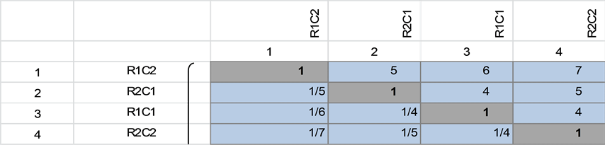
The output from the template in Figure 1 is the important pairwise comparison matrix. All criteria compared to themselves get a value of 1. We obtained the following AHP matrix:
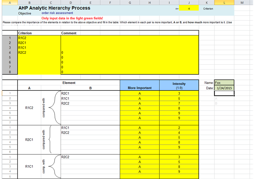
Figure 1. AHP template.
From this matrix, we determine the eigenvalues and associated eigenvectors. We get weights (eigenvector) of the following (to 3 decimals)
x = 0.595
w = 0.211
y = 0.122
z = 0.071
Player 2
C1 C2
Player 1 R1 0.211 0.595
R2 0.122 0.071
The solution, regardless of the numbers put in for w, x, y, or z is the value in R1C2. The major difference is that the method using AHP is based on real preferences not ordinal preferences. Thus, AHP can help obtain the relative values of the outcomes provided the CR < 0.1. The resulting values are the cardinal utilities values based upon the input preferences. For example, we may conclude here that R1C2 is 4.877 (0.595/0.122) times as important than R2C1.
5. AHP Example in Game Theory
In our game theory course, we initially cover ordinal utility as a method to obtain values for a payoff matrix. Let’s apply this to two-person non-zero sum game example from the course.
Example 1. Unites States versus Country X
Consider a game between two players with two strategies each where the best we can initially do is to obtain an ordinal ranking their preferences. The game payoff matrix is listed in Table 3.
There are no pure strategies so the players must play equalizing or mixed strategies to find the equilibrium. We find that we are stuck because these are ordinal values. In the past, our students just assume that these values are in fact cardinal values. With that assumption, we find the United States Play ¼ R1 and ¾ R2 while Country X plays ¾ C1 and ¼ C2. The Nash equilibrium is (2.5, 2.5). Further, if we find Prudential strategies, the Securi-
Table 3. Ordinal payoff matrix.
ty Values, to get to Nash Arbitration [11] with these values we find that the United States plays ½ R1, ½ R2 with a security value of 2.5 while Country X plays ½ C1, ½ C2 with a security value of 2.5. Using (2.5, 2.5) we find the Nash Arbitration values are (2.75, 2.875) while playing 3/8 of R1C2 and 5/8 of R1C1, as displayed in Figure 2 using the AHP method [10] [11] .
The issue is “what does the Nash arbitration mean” since the initial values were merely ordinal values with no indication how much better a 4 is than a 3, 2, or 1 for each player.
Rather than use the Lottery Method suggested by Morgenstern and von Neumann, we suggest the pairwise comparison method of Saaty for each player’s strategies combination. For both the United States and Country X we will need cardinal values for their preferences with these combined strategies: R1C1, R1C2, R2C1, and R2C2.
First, we use Saaty’s method [8] for the United States. We utilize a template build for class work [10] [11] . Figure 2 shows the intensity of the pairwise comparisons for our example with a CR = 0.0899, which is less than 0.1.
The pairwise comparison matrix is
For the U.S., using this matrix, we obtain the following eigenvector as our cardinal values .
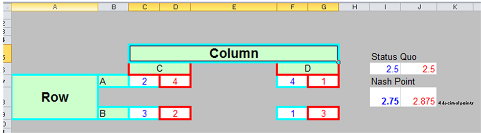
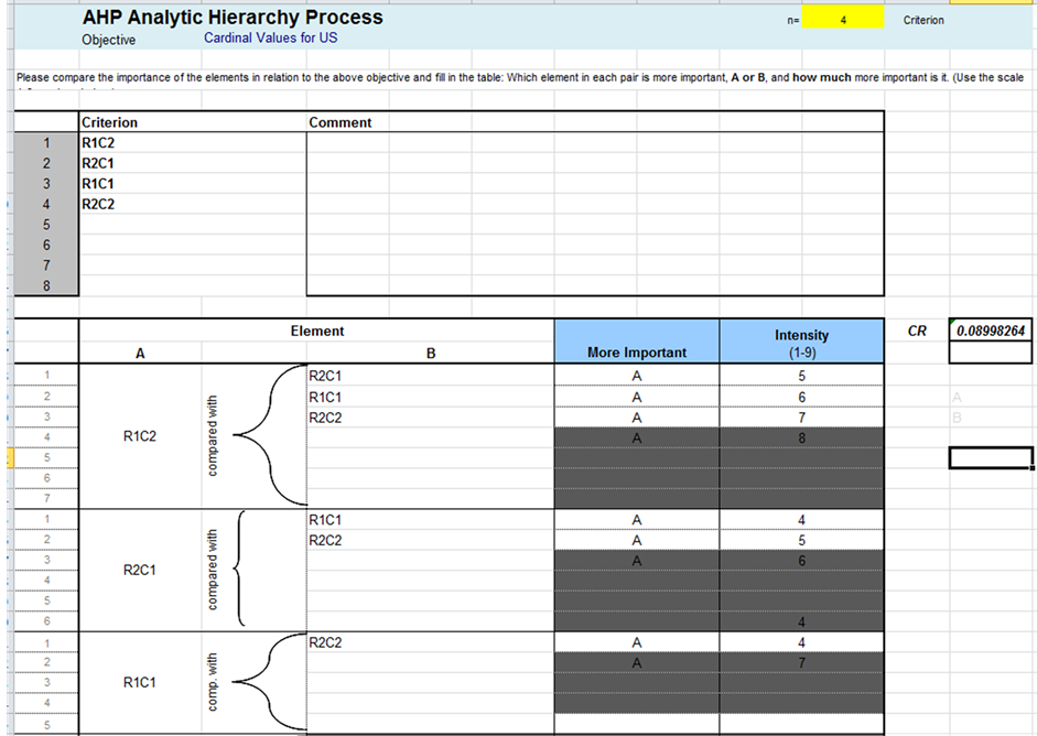
Figure 2. Pairwise comparisons for the United States.
For Country X, we obtain cardinal values as shown by obtaining the intensity of the pairwise comparisons shown in Figure 3 with a CR = 0.0569, which is less than 0.1. Next, we obtain the eigenvector of the pairwise comparison matrix.
The pairwise comparison matrix is:
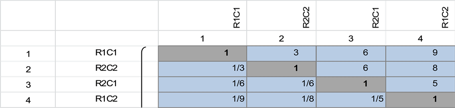
The cardinal values, the eigenvector, of the pairwise comparison matrix for Country X are as follows
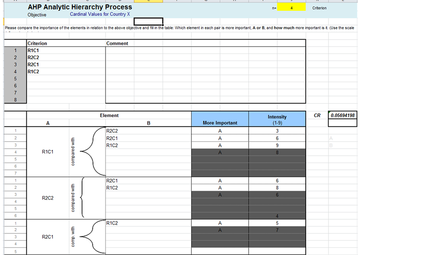
Figure 3. Pairwise comparisons for Country X.
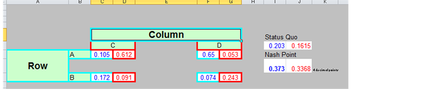
The entire game theory payoff matrix, with cardinal values representing true preferences, is displayed in Table 4.
The Nash Equilibrium, Prudential Strategies, and the Nash Arbitration are found using templates built for classroom use [12] and displayed. We find the Nash equilibrium (0.202619, 0.16153).
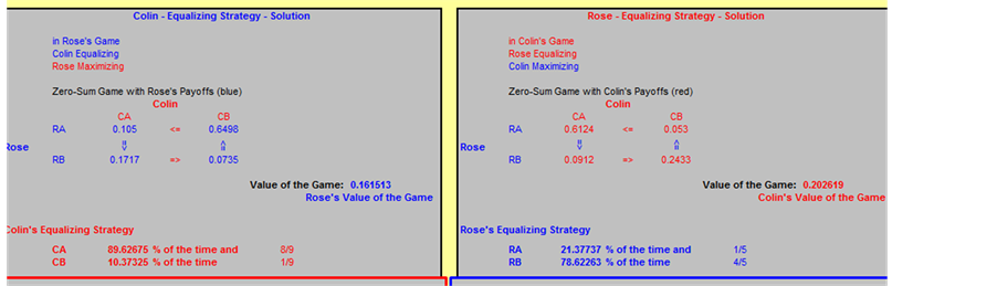
We find the Prudential Strategies or Security Levels are the Nash equilibrium from before.
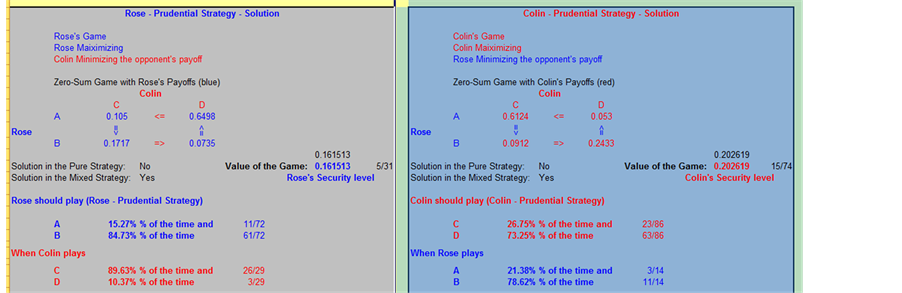
Table 4. Cardinal payoff matrix using AHP results.
Table 5. Summary results.
We find the Nash Arbitration (0.373, 0.3368) by playing 0.5075 of R1C1 and 0.4925 of R1C2.
We see that our mixed strategies probabilities are different with cardinal preferences than they were with the ordinal preferences that we merely assumed were cardinal preferences. We have had cases where the decisions in AHP and game theory are altered through the use of this method to obtain cardinal values as well as sensitivity analysis of the cardinal weights.
6. Summary and Conclusions
We have showed that differences in playing strategies in game theory occur as a function of the values in the payoff matrix. Table 5 displays a comparative summary for our example.
In conclusion, not only did the numerical values change but also two key points were seen in this example. First, using cardinal values, the Nash arbitration favored the United States whereas before it favored Country X. Second, how we played our strategies in the game changed substantially.
References
- Straffin, P. (2004) Game Theory and Strategy. The Mathematical Association of America: New Mathematics Library, Washington DC.
- Fox, W. and Everton, S. (2013) Mathematical Modeling in Social Network Analysis: Using TOPSIS to Find Node Influences in a Social Network. Journal of Mathematics and Systems Science, 3, 531-541.
- Fox, W. and Everton, S. (2014) Mathematical Modeling in Social Network Analysis: Using Data Envelopment Analysis and Analytical Hierarchy Process to Find Node Influences in a Social Network. Journal of Defense Modeling and Simulation, 2014, 1-9.
- Fox, W. and Everton, S.F. (2014) Using Mathematical Models in Decision Making Methodologies to Find Key Nodes in the Noordin Dark Network. American Journal of Operations Research, 1-13 (Online).
- Fox, W. and Thompson, M.N. (2014) Phase Targeting of Terrorist Attacks: Simplifying Complexity with Analytical Hierarchy Process. International Journal of Decision Sciences, 5, 57-64.
- Fox, W.P. (2014) Phase Targeting of Terrorist Attacks: Simplifying Complexity with TOPSIS. Journal of Defense Management, 4, 116. http://dx.doi.org/10.4172/2167-0374.1000116
- Fox, W.P. (2014) Using Multi-Attribute Decision Methods in Mathematical Modeling to Produce an Order of Merit List of High Valued Terrorists. American Journal of Operation Research, 4, 365-374. http://dx.doi.org/10.4236/ajor.2014.46035
- Saaty, T. (1980) The Analytical Hierarchy Process. McGraw Hill, New York.
- Alinezhad, A. and Amini, A. (2011) Sensitivity Analysis of TOPSIS Technique: The Results of Change in the Weight of One Attribute on the Final Ranking of Alternatives. Journal of Optimization in Industrial Engineering, 7, 23-28.
- Fox, W.P. (2012) Mathematical Modeling of the Analytical Hierarchy Process Using Discrete Dynamical Systems in Decision Analysis. Computers in Education Journal, 3, 27-34.
- Fox, W. (2014) Chapter 221, TOPSIS in Business Analytics. Encyclopedia of Business Analytics and Optimization, V, 281-291.
- Feix, M. (2007) Game Theory: Toolkit and Workbook for Defense Analysis Students. MS Thesis, Naval Postgraduate School, Monterey.
Biographical Sketch
Dr. William P. Fox is a professor in the Department of Defense Analysis at the Naval Postgraduate School and teaches a three course sequence in mathematical modeling for decision making. He received his BS degree from the United States Military Academy at West Point, New York, his MS at the Naval Postgraduate School, and his Ph.D. at Clemson University. Previous he has taught at the United States Military Academy and Francis Marion University where he was the chair of mathematics for eight years. He has many publications and scholarly activities including books, chapters of books, journal articles, conference presentations, and workshops. He directs several mathematical modeling contests through COMAP: the HiMCM and the MCM. His interests include applied mathematics, optimization (linear and nonlinear), mathematical modeling, statistical models for medical research, multi-attribute decision making, game theory, and computer simulations. He is president-emeritus of the NPS faculty council. He is currently Past President of the Military Application Society of INFORMS.