American Journal of Operations Research
Vol.4 No.4(2014), Article
ID:48100,13
pages
DOI:10.4236/ajor.2014.44025
Using Mathematical Models in Decision Making Methodologies to Find Key Nodes in the Noordin Dark Network
William P. Fox, Sean F. Everton
Department of Defense Analysis, Naval Postgraduate School, Monterey, USA
Email: wpfox@nps.edu, sfeverton@nps.edu
Copyright © 2014 by authors and Scientific Research Publishing Inc.
This work is licensed under the Creative Commons Attribution International License (CC BY).
http://creativecommons.org/licenses/by/4.0/
![]()
![]()

Received 20 May 2014; revised 25 June 2014; accepted 3 July 2014
ABSTRACT
A Dark Network is a network that cannot be accessed through tradition means. Once uncovered, to any degree, dark network analysis can be accomplished using the SNA software. The output of SNA software includes many measures and metrics. For each of these measures and metric, the output in ORA additionally provides the ability to obtain a rank ordering of the nodes in terms of these measures. We might use this information in decision making concerning best methods to disrupt or deceive a given dark network. In the Noordin Dark network, different nodes were identified as key nodes based upon the metric used. Our goal in this paper is to use methodologies to identify the key players or nodes in a Dark Network in a similar manner as we previously proposed in social networks. We apply two multi-attribute decision making methods, a hybrid AHP & TOPSIS and an average weighted ranks scheme, to analyze these outputs to find the most influential nodes as a function of the decision makers’ inputs. We compare these methods by illustration using the Noordin Dark Network with seventy-nine nodes. We discuss sensitivity analysis that is applied to the criteria weights in order to measure the change in the ranking of the nodes.
Keywords:Social Network Analysis, Multi-Attribute Decision Making, Analytical Hierarchy Process (AHP), Decision Criterion, Weighted Criterion, TOPSIS, Node Influence, Sensitivity Analysis, Average Weighted Ranks

1. Introduction to Dark Networks
Social Network Analysis (SNA) is the methodical analysis of social networks in general and dark networks [1] . Social network analysis is a collection of theories and methods that assumes that the behavior of actors (individuals, groups, organizations, etc.) is profoundly affected by their ties to others and the networks in which they are embedded. Rather than viewing actors as automatons unaffected by those around them, SNA assumes that interaction patterns affect what actors say, do, and believe. Networks contain nodes (representing individual actors or entities within the network) and edges and arcs (representing relationships between the individuals, such as friendship, kinship, organizational position, sexual relationships, communications, tweets, Facebook friendships, terrorists, etc.). These networks are often depicted in two formats: graphically or matrix. We might call the graph a social network diagram or dark network diagram, where nodes are represented as points or circles and arcs are represented as lines that interconnect the nodes.
A Dark Network is any network organization that cannot be assessed by typical means. These might include drug cartels, alien smuggling rings, money laundering operations, terrorism, illegal trafficking, and nuclear proliferation. According to Milward [2] [3] , the ideal type dark network is both covert and illegal. In reality, many networks are deemed “gray” networks. We assume that the things that make a network effective for legal activities also makes them effective for illegal activities. Therefore, we propose to apply the same mathematical modeling proposal at Dark Networks as we did to Social Networks in previous studies.
In their article, Millward [2] [3] also proposed the question, “Can understanding legal network help in understanding dark networks?” Their research shows it can help as they applied this to the 9 - 11 terrorist network and other dark networks.
We will provide a brief background of social network analysis. More precisely, we introduce some of the more common metrics and measures as well as their definitions that are used for exploratory analysis of networks. In this paper, we assume decision makers are only looking for the powerful and influential players in a network. In the SNA literature, there has been some discussion as to four main measures that might be used to analysis the most influential person in a network [4] and these include only the following centrality measures: degree centrality, betweenness, closeness, and eigenvector. In our research, we use all eight output metrics and then only the four key metric to see the impact of using only four versus the eight metrics.
There are a multitude of measures (metrics) that are found in most SNA software. The software package that we used in this analysis is ORA [5] :
We begin by defining the main four centrality metrics. Other metric definitions may be seen in social network literature [6] -[8] .
Betweenness: Betweenness is a measure of the extent to which a node lies on the shortest path between other nodes in the network. This measure takes into account the connectivity of the node’s neighbors, giving a higher value for nodes which bridge clusters. The measure reflects the number of people who a person is connecting indirectly through their direct links.
Closeness: Closeness is the degree an individual is near all other individuals in a network (directly or indirectly). It reflects the ability to access information through the “grapevine” of network members. Thus, closeness is the inverse of the sum of the shortest distances between each individual and every other person in the network. The shortest path may also be known as the “geodesic distance”.
Eigenvector Centrality: Eigenvector centrality is a variation on degree centrality in that assumes that ties to central actors are more important than ties to peripheral actors and thus weights an actor’s summed connections to others by their centrality scores. Google’s Page Rank score is a variation on eigenvector centrality.
Degree Centrality: Degree centrality is defined as the number of links incident upon a node (i.e., the number of ties that a node has). The degree can be interpreted in terms of the immediate risk of a node for catching whatever is flowing through the network (such as a virus, or some information). In the case of a directed network (where ties have direction), we usually define two separate measures of degree centrality, namely indegree and outdegree.
For our analysis, we use the subset of the Noordin Top Terrorist Network drawn primarily from “Terrorism in Indonesia: Noordin’s Networks”, a 2006 publication of the International Crisis Group. It includes relational data on the 79 individuals listed that publication. The data were initially coded by Naval Postgraduate School students and the Common Research Environmental (CORE) Lab in our department.
Previous works on using AHP and TOPSIS [7] [8] have shown the proof of principle approach using two basic social networks from the literature and applied methods for obtaining the eigenvectors using dynamical systems [9] [10] and power methods [11] .
2. Methodologies to Find Key Players across Many Metrics: Application of Technique of Order Preference by Similarity to the Ideal Solution (TOPSIS) in a Dark Network
The Technique for Order of Preference by Similarity to Ideal Solution (TOPSIS) is a multi-attribute decision analysis method [12] -[14] that continues to be widely used to rank order alternatives. TOPSIS is based on the concept that the chosen alternative should have the shortest geometric distance from the positive ideal solution and the longest geometric distance from the negative ideal solution. It is a method of compensatory aggregation that compares a set of alternatives by identifying weights for each criterion, normalizing the scores for each criterion based upon the TOPSIS normalization design and calculating the geometric distance between each alternative and the ideal alternative, which is the best score in each criterion. An assumption of TOPSIS is that the criteria are monotonically increasing or decreasing.
Compensatory methods such as TOPSIS allow trade-offs between criteria, where a poor result in one criterion can be negated by a good result in another criterion. This provides a more realistic form of modeling than noncompensatory methods, which include or exclude alternative solutions based on hard cut-offs.
2.1. TOPSIS Background
We only desire to briefly discuss the elements in the framework of TOPSIS. TOPSIS can be described as a method to decompose a problem into sub-problems. In most decisions, the decision maker has a choice among several to many alternatives. Each alternative has a set of attributes or characteristics that can be measured, either subjectively or objectively. The attribute elements of the hierarchal process can relate to any aspect of the decision problem—tangible or intangible, carefully measured or roughly estimated, wellor poorly-understood—anything at all that applies to the decision at hand.
The TOPSIS process is carried out in the following seven steps described as follows:
Step 1 Create an evaluation matrix consisting of m alternatives and n criteria, with the intersection of each alternative and criteria given as xij, giving us a matrix .
.
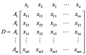
Step 2 The matrix shown as D above then normalized to form the matrix , using the normalization method

for i = 1, 2···, m; j = 1, 2,··· n.
Step 3 Calculate the weighted normalized decision matrix. First, we need the weights. Weights can come from either the decision maker or by computation using a scheme such as AHP with the pairwise comparisons [15] . The sum of the weights over all attributes must equal 1 regardless of the method used. Multiply the weights to each of the column entries in the matrix from Step 2 to obtain the matrix, T.

Step 4 Determine the worst alternative (Aw) and the best alternative (Ab): Examine each attribute’s column and select the largest and smallest values appropriately. If the values imply larger is better (profit) then the best alternatives are the largest values and if the values imply smaller is better (such as cost) then the best alternative is the smallest value.


where  associated with the criteria having a positive impact, and
  associated with the criteria having a negative impact.
We suggest that if possible make all entry values in terms of positive impacts.
Step 5 Calculate the L2-distance between the target alternative i and the worst condition Aw
 and the distance between the alternative i and the best condition Ab
 where diw and dib are L2-norm distances from the target alternative i to the worst and best conditions, respectively.
Step 6 Calculate the similarity to the worst condition:
 .
.
Siw = 1 if and only if the alternative solution has the worst condition; and Siw = 0 if and only if the alternative solution has the best condition.
Step 7 Rank the alternatives according to their value from .
.
2.2. TOPSIS Uses and Applications
While TOPSIS can be used by individuals working on straightforward decisions, TOPSIS is most useful where teams of people are working on complex problems, especially those with high stakes, involving human perceptions and judgments, whose resolutions have long-term repercussions. It has unique advantages when important elements of the decision are difficult to quantify or compare, or where communication among team members is impeded by their different specializations, terminologies, or perspectives.
Decision situations to which the TOPSIS might be applied include:
• Choice―The selection of one alternative from a given set of alternatives, usually where there are multiple decision criteria involved.
• Ranking―Putting a set of alternatives in order from most to least desirable.
• Prioritization―Determining the relative merit of members of a set of alternatives, as opposed to selecting a single one or merely ranking them.
• Resource allocation―Apportioning resources among a set of alternatives.
• Benchmarking―Comparing the processes in one's own organization with those of other best-of-breed organizations.
• Quality management―Dealing with the multidimensional aspects of quality and quality improvement.
• Conflict resolution―Settling disputes between parties with apparently incompatible goals or positions.
3. Applications to Noordin Dark Network
We will illustrate using the Noordin Dark Network with graphical network depicted in Figure 1.
We obtained all the outputs from ORA and a summary of Key Node analysis as shown in Table1 Table 1 shows different key nodes across the metrics. The four main centralities are italicized.
We extracted the actual metric values from the output of ORA for the 20 nodes across these key metrics. Table 2 provides these metrics values from ORA for the top 20 nodes (size: 79 nodes, density: 0.0879585) for eight outputs initially identified by ORA. First, we performed analysis using all eight metric as decision criteria. Next, we performed the analysis with only the main four centrality measures as decision criteria.
We use the decision weights from our AHP template program (unless a real decision maker gives us their own weights) and find the eigenvectors for our eight metrics as shown in Table 3 displaying the pairwise comparison,
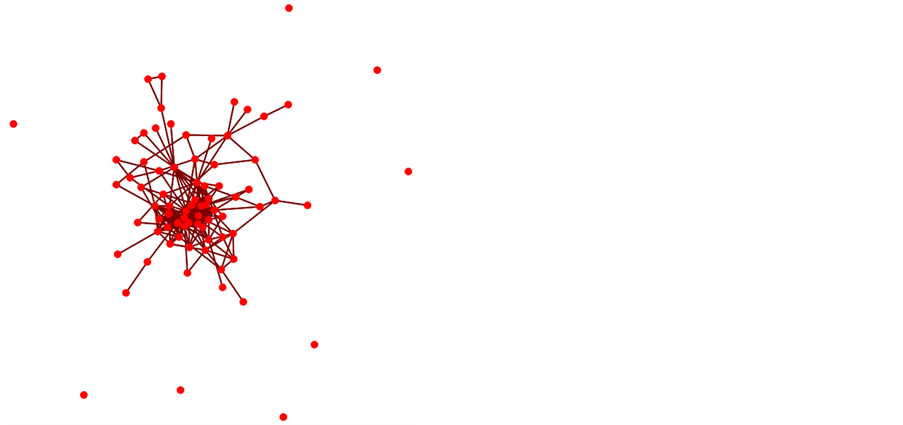
Figure 1. ORA’s trust network from noordin’s seventy-nine node dark network.

Table 1. ORA’s key nodes from the Noordin Dark Network.
Table 2. Summary of ORA’s output for Noordin Dark Network for the 8 criterion.
Table 3. Decision pairwise matrix and decision weights.
the consistency ratio (CR must be less than 0.1) and the resulting eigenvectors [16] .
We take all these output metrics from ORA and perform steps 2 - 7 of TOPSIS to obtain the following raw and then ordered outputs shown in Table4
We repeated the analysis using only the four main centrality measures. Table 5 shows the decision matrix and weights with a CR = 0.02846 (which is less than 0.1).
Table 4. Raw and ordered outputs from TOPSIS.
Table 5. Decision matrix and weights with four key metrics.
Table 6 shows the raw and ordered TOPSIS output.
We note that the top 5 nodes do not change their order and the first change occurs in position number 6.
4. Sensitivity Analysis
In our analysis, we have utilized weights as applicable to the metrics for the nodes. Weights are subjective, based upon the pairwise comparisons, even if used in AHP and TOPSIS methodologies. The literature provides no direct sensitivity analysis procedures. We recommend, as a minimum, at least a numerical trial and error approach to sensitivity analysis. Not only do we recommend altering the criterion pairwise comparison to measure the model’s robustness but also delving into break points is proven to be useful.
In our four-metric model, we find that the model is quite robust and that with major changes in priority and pairwise comparison the top 5 nodes are not affected see Figure 2. We used the formula recommended [17] for adjusting decision maker weights as Equation (1):
Table 6. Raw and ordered outputs from TOPSIS.
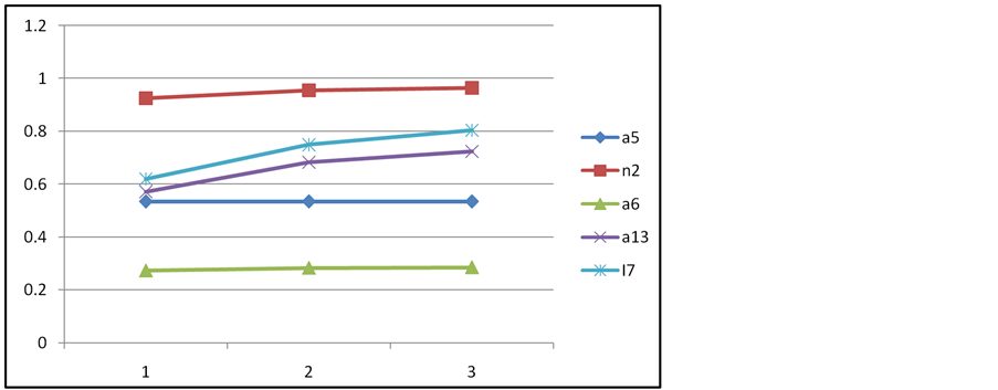
Figure 2. Sensitivity analysis on the 4 criteria model top 5 with substantial changes to criterion weighting.
 (1)
(1)
where ![]() is the new weight and wp is the original weight of the criterion to be adjusted and
is the new weight and wp is the original weight of the criterion to be adjusted and ![]() is the value after the criterion was adjusted.
is the value after the criterion was adjusted.
In the eight-metric model, we again used the formula recommended [17] for adjusting decision maker weights. We plotted the top 10 alternatives using three major adjustments in criteria weighting each time insuring a different criterion was the most heavily weighted. It is seen from the graph, Figure 3, that the top 5 never changed position.
Finding Break Points, if They Exist
A break point is defined as the value of weight, ![]() , that causes the ranking to be significantly change implying a change in the top alternative ranking. The method that we suggest is taking the largest weighted criterion and reduces it is slight increments which increases the weights of the other criteria and re-computing the rankings until another alternative is ranked number one.
, that causes the ranking to be significantly change implying a change in the top alternative ranking. The method that we suggest is taking the largest weighted criterion and reduces it is slight increments which increases the weights of the other criteria and re-computing the rankings until another alternative is ranked number one.
In this examination, the top ranked node, n2, never changes as shown in Figure 4. We can get changes in the nodes ranked 2 - 4 through an increase change in the criterion weight for closeness centrality from 0.1611 to 0.4611, an increase of 0.3.
5. Average Weighted Ranks
Recall that Table 1 provided the top 20 ranks by SNA metrics, our criteria. We took the nodes and replaced the value under each metric with their rank in the top 20. We gave a missing value to ranks for nodes outside the top 20. There are two schemes that can be used here where each results the lower the overall rank the more influential the node. The first, is equal weighting of all metrics and then average the final ranks from 1 - 20 and shown in Table7 The second, using the AHP weights from before, to weight the ranks by the importance of the criteria shown in Table8
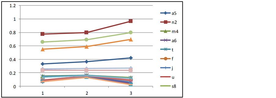
Figure 3. Sensitivity analysis.
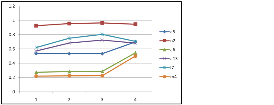
Figure 4. Looking for break points
Table 7. Average ranks of nodes over the eight criteria.
We suggest sensitivity analysis could also be applied to this technique by using Equation (1) to change the weights.
6. Summary and Comparisons
We compare our MADM analysis with an average priority method using the information proved in Table 1 where we transformed the node to a ranking position 1 - 20 and a complete AHP process. We present our results in the following Table9 We find the node n2 is ranked number one is all methods except the average ranking from Table 1 that indicated that A5 is the top node.
Table 8. Weighted average ranks.
We compared the results and find they are similar. We have provided several approaches to ranking influential nodes (players) in a given social network. We have illustrated using the Noordin Dark Network with 79 nodes and found that nodes A5 and N2 were clearly always in the top. We believe that the incorporation of decision maker weights with the metrics of a given dark or social network is invaluable to analysis of key and influential players.
Table 9. Summary of multiple MADM methods applied to Noordin 79 node Dark Network.
Acknowledgements
This research received no specific grant from any funding agency in the public, commercial, or not-for-profit sectors. This work reflects the research of the authors and does represent the opinions of the Department of Defense, the Department of the Navy, or The Naval Postgraduate School. We thank the reviewers for the comments and suggestions.
References
- Everton, S. and Roberts, N. (2011) Strategies for Combating Dark Networks. Journal of Social Structure, 12, 1-32.
- Milward, H.B. and Raab, J. (2003) Dark Networks as Problems. Journal of Public Administration Research and Theory, 13, 413-439. http://dx.doi.org/10.1093/jopart/mug029
- Milward, H.B. and Raab, J. (2003) Dark Networks as Problems. Paper Presented to the 8th Public Management Research Conference at the School of Policy, Planning and Development at University of Southern California, Los Angeles, 29 September-1 October 2005.
- Newman, M. (2010) Networks: An Introduction. Oxford University Press, Oxford.http://dx.doi.org/10.1093/acprof:oso/9780199206650.001.0001
- Carley, K. (2001-2011) Organizational Risk Analyzer (ORA). Carnegie Mellon University, Center for Computational Analysis of Social and Organizational Systems (CASOS), Pittsburgh.
- Everton, S. (2012) Disrupting Dark Networks. Cambridge University Press, Cambridge, UK and New York, USA.http://dx.doi.org/10.1017/CBO9781139136877
- Fox, W. and Everton, S. (2014) Using Data Envelopment Analysis and the Analytical Hierarchy Process to Find Node Influences in a Social Network. Journal of Defense Modeling and Simulation, 11, 1-9.
- Fox, W. and Everton, S. (2013) Mathematical Modeling in Social Network Analysis: Using TOPSIS to Find Node Influences in a Social Network. Journal of Mathematics and System Science, 3, 531-541.
- Fox, W. (2102) Mathematical Modeling of the Analytical Hierarchy Process Using Discrete Dynamical Systems in Decision Analysis. Computers in Education Journal, 22, 27-34.
- Giordano, F., Fox, W. and Horton, S. (2103) A First Course in Mathematical Modeling. 5th Edition, Brooks-Cole Publishers, Boston.
- Burden, R. and Faires, D. (2011) Numerical Analysis. 9th Edition, Brooks-Cole Publishers, Boston.
- Huang, I., Keisler, J. and Linkov, I. (2011) Multi-Criteria Decision Analysis in Environmental Science: Ten Years of Applications and Trends. Science of the Total Environment, 409, 3578-3594.http://dx.doi.org/10.1016/j.scitotenv.2011.06.022
- Hwang, C. and Yoon, K. (1981) Multiple Attribute Decision Making: Methods and Applications. Springer-Verlag Publishers, New York. http://dx.doi.org/10.1007/978-3-642-48318-9
- Hwang, C., Lai, Y. and Liu, T. (1993) A New Approach for Multiple Objective Decision Making. Computers and Operational Research, 20, 889-899. http://dx.doi.org/10.1016/0305-0548(93)90109-V
- Yoon, K. (1987) A Reconciliation among Discrete Compromise Situations. Journal of Operational Research Society, 38, 277-286. http://dx.doi.org/10.1057/jors.1987.44
- Satty, T. (1980) The Analytical Hierarchy Process. McGraw Hill, New York.
- Alinzhad, A. and Amini, A. (2011) Sensitivity Analysis of TOPSIS Technique: The Results of Change in the Weight of One Attribute on the Final Ranking of Alternatives. Journal of Optimization in Industrial Engineering, 7, 23-28.