American Journal of Operations Research
Vol. 2 No. 2 (2012) , Article ID: 19939 , 10 pages DOI:10.4236/ajor.2012.22024
A Genetic Algorithm for the Split Delivery Vehicle Routing Problem
1Industrial and Information Engineering Department, University of Tennessee, Knoxville, USA
2Industrial and Manufacturing Engineering Department, Pennsylvania State University, University Park, USA
Email: jwilck@utk.edu, tmc7@psu.edu
Received February 18, 2012; revised March 20, 2012; accepted April 5, 2012
Keywords: Vehicle Routing Problem; Transportation; Genetic Algorithm
ABSTRACT
The Split Delivery Vehicle Routing Problem (SDVRP) allows customers to be assigned to multiple routes. Two hybrid genetic algorithms are developed for the SDVRP and computational results are given for thirty-two data sets from previous literature. With respect to the total travel distance and computer time, the genetic algorithm compares favorably versus a column generation method and a two-phase method.
1. Introduction
The basic model for this paper is a vehicle routing problem (VRP) variant, the split delivery vehicle routing problem (SDVRP). Standard forms of the VRP have been studied for decades as shown in the seminal paper by Dantzig and Ramser [1] and an algorithm developed by Clarke and Wright [2]. Recent surveys by Toth and Vigo [3] and Cordeau et al. [4,5] examine exact and heuristic procedures of the VRP, respectively. Golden and Assad [6] and Toth and Vigo [7] edited books solely devoted to the VRP and its variants, and Laporte and Osman [8] provide an extensive bibliography. Reimann [9] analyzed a vehicle routing problem with stochastic demands.
The SDVRP is appropriate for many CVRP applications where customers can be visited more than once. Numerous applications for the CVRP are noted in the literature [6,7], with the primary emphasis being the distribution of various goods. Dror and Trudeau [10,11] formally introduced the SDVRP. The primary motivation to split a customer’s demand over multiple routes is to reduce the travel distance and the number of vehicle routes. If each vehicle has the same capacity, then the minimum number of routes is the total demand divided by the vehicle capacity rounded up to the nearest integer.
Genetic algorithms have been used in a variety of areas [12]. There applications have been noted in many industrial engineering areas, including scheduling [13], vehicle routing [14], and the generalized orienteering problem [15].
2. Literature Review
2.1. Split Delivery Vehicle Routing Problem Literature Review
Dror and Trudeau [10,11] formally introduced the SDVRP. The primary motivation to split a customer’s demand over multiple routes is to reduce the travel distance and the number of vehicle routes. If each vehicle has the same capacity, then the minimum number of routes is the total demand divided by the vehicle capacity rounded up to the nearest integer. They proved, given that the distance between nodes follows the triangle inequality, there exists an optimal solution where no two routes can have more than one split demand point in common, and that there exists an optimal solution with no k-split cycles (for any k). Based on these proofs, Dror and Trudeau [11] devised a heuristic to solve the SDVRP given an initial CVRP solution by splitting a node’s demand to fill the routes to capacity. Dror et al. [16] extended the formulation of Dror and Trudeau [10,11] with additional constraints, and developed a constraint relaxation branch and bound algorithm. The results from Dror and Trudeau [10, 11] and Dror et al. [16] show that the percent reduction in travel distance, when compared to the CVRP, is most prominent among problems where customers have high demands (i.e., more than 10% of the vehicle capacity). The results showed that the SDVRP solution used fewer routes than the CVRP solution; however, the SDVRP solution did not always use the minimum number of routes.
Frizzell and Giffin [17,18] solved the SDVRP with time windows on grid networks and developed heuristics to generate solutions. Archetti et al. [19] and Aleman and Hill [20] developed tabu search procedures for the SDVRP. Archetti et al. [21] analyzed the worst-case properties of the SDVRP. Archetti et al. [22] discussed when demand splitting is most beneficial. Lee et al. [23] developed a dynamic programming model for the vehicle routing problem with split pick-ups with an uncountable (infinite) number of state and action spaces. Belenguer et al. [24] performed a polyhedral study on the SDVRP to produce lower bounds through formulating the problem with undirected arcs by assuming symmetric distances. Using a cutting-plane algorithm in conjunction with a relaxed formulation, they were able to obtain feasibility gaps within 12% for problems with 50, 75, and 100 customers. Jin et al. [25] developed a two-stage algorithm to solve the SDVRP using valid inequalities. Jin et al. [26,27] presented a column generation procedure that provides comparable lower and upper bounds for the data sets developed by Belenguer et al. [24]. Chen et al. [28] presented a mixed integer program and a variable length record-to-record travel algorithm. Burrows [29] showed that the SDVRP could be modified by splitting customer demand into smaller quantities on the same node, and then solved using CVRP methods. Wilck and Cavalier [30] developed a construction heuristic to quickly generate feasible solutions to the SDVRP. Aleman et al. [31] present an adaptive memory algorithm for the SDVRP. Archetti and Speranza [32] and Gulczynski et al. [33] recently surveyed the SDVRP literature. Recent theses addressing the SDVRP include Aleman [34], Wilck [35], Liu [36], Nowak [37], and Chen [38].
Direct applications of the SDVRP have been noted in literature. Mullaseril et al. [39] modeled a cattle feed distribution problem as an SDVRP with time windows. Sierksma and Tijssen [40] model a helicopter crewscheduling problem using an SDVRP model, developed a relaxed linear program and column generation scheme to find a solution, and used a cluster-and-route procedure. Song et al. [41] modeled a newspaper distribution process as a SDVRP and solved using a two-phase procedure. The first phase allocates customers using a binary program and the second phase generates vehicle routes.
2.2. Genetic Algorithms in Vehicle Routing Problems Literature Review
A genetic algorithm is a global search procedure that solves problems by emulating evolution. A pure genetic algorithm uses reproduction and mutation to develop a new generation of solutions from the current generation of solutions. The constraints of the VRP do not allow the application of pure genetic algorithms without an additional step to ensure feasibility.
The book by Goldberg [42] describes the solution process of genetic algorithms. The Fundamental Theorem of Genetic Algorithms states the conditions in order to achieve a global optimal solution [43]. These conditions describe the breeding process and insist that better solutions (or patterns) remain in future generations while weaker solutions (or patterns) are eliminated from future generations. The typical genetic algorithm follows these basic steps [43].
The procedure outlined here is a basic genetic algorithm. Procedures for generating feasible offspring and feasibly mutating the new generation are problem-specific. For example, given a problem that can be represented by a binary string with four values. Then the following example can occur: Parent 1: 0-1-1-0 and Parent 2: 1-0-1-1.
A crossover will occur between any of the four values (i.e., between the first and second, between the second and third, and between the third and fourth). Based on probability (e.g., generating a random number between 0 and 1), the crossover point is chosen as between the second value and the third value. Thus the crossover will take 0-1 from Parent 1 and switch it with 1-0 from Parent 2, resulting in two offspring: Child 1: 1-0-1-0 and Child 2: 0-1-1-1. The mutation stage will then, using probability, randomly select a small number of offspring (if any at all) and change a small portion of position values. For example, suppose that based on probability, Child 2 is to be mutated in the second position. Originally, Child 2 is 0-1-1-1; and with mutation she is 0-0-1-1.
The preceding example assumed a binary string problem structure with no limiting constraints. Unfortunately, applying genetic algorithms directly to VRP variants is difficult due to the constraints of the problems. Therefore, additional steps or changes are necessary to ensure feasibility of created solutions. For VRP variants the reproduction stage (i.e., Step 4) can be modified to ensure feasible solutions or an additional step can be added after the mutation stage (i.e., Step 5) to fix infeasible solutions.
Gendreau et al. [44] described three approaches to the VRP with time windows, where each approach ensures feasibility differently. The first approach ensures feasibility while sacrificing the evolutionary aspects of the genetic algorithm; thus, it is considered a hybrid approach. This approach does not allow infeasible reproduction or mutation. The second approach applies a genetic algorithm to the partitioning of customers to routes, but the routes are solved separately to ensure feasibility. The third approach applies a genetic algorithm directly, but incorporates a post-processing step to ensure feasibility. The third approach yielded the best results in terms of the objective; however, it was computationally expensive. Gendreau et al. [45] stated that accounting for the constraints of the VRP makes a genetic algorithm computationally expensive.
Alvarenga et al. [14] developed a two-phase approach for the VRP with time windows by using a hybrid genetic algorithm and a set-partitioning method to generate routes. The two-phase approach yielded good solutions when compared to best known solutions. Solution time was not compared or reported, but the genetic algorithm was given a time limit of 60 minutes.
Baker and Ayechew [46] developed a pure genetic algorithm and a hybrid genetic algorithm for the CVRP while constraining the maximum distance of a route. The pure genetic algorithm produced poor solutions, when compared to previous simulated annealing and tabu search methods. The hybrid genetic algorithm provided comparable, although not superior, solutions when compared to previous methods in a reasonable amount of computer time. The hybrid genetic algorithm applied neighborhood search procedures to ensure a feasible solution.
Wang et al. [15] developed a genetic algorithm for the generalized orienteering problem. The orienteering problem is a VRP variant where a start point and an end point are specified and other points have associated scores. The objective is to determine a path that maximizes the score while adhering to a time constraint. The generalized orienteering problem (GOP) adds a level of complexity where there are numerous attributes at a specific point that represent the total score. The GOP is similar to a VRP with one vehicle route. The genetic algorithm developed by Wang et al. [15] compared favorably to an artificial neural network solution procedure. The genetic algorithm procedure initially allowed infeasible solutions, but then corrected the solutions by truncating them to accommodate the time constraint.
Jeon et al. [47] consider the VRP with multiple depots and up to two deliveries per node (i.e., split delivery). They developed a pure genetic algorithm and a hybrid genetic algorithm. The hybrid genetic algorithm ensured that no infeasible solutions were generated, and the hybrid genetic algorithm provided consistently better results in terms of objective value. Computation time was not provided for the pure genetic algorithm.
2.3. Data Sets from Previous Literature
Data sets from Belenguer et al. [24] and Chen et al. [28] were used to test the hybrid genetic algorithm procedure presented in this paper. The procedure was coded in FORTRAN 95 and compiled by GNU FORTRAN on an Intel Xeon Processor 2.49 GHz computer with 8 GB RAM. The number of customers and vehicles for 11 data sets from Belenguer et al. [24] are shown in Table 1. The number of customers ranged from 50 to 100, with an additional node for the depot. The data sets also differ by
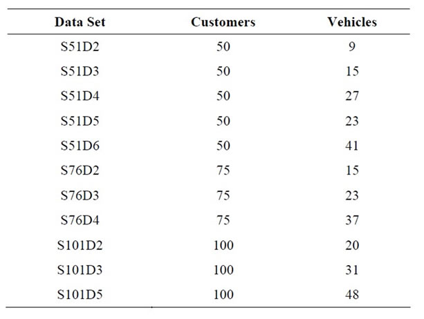
Table 1. Eleven data sets from Belenguer et al. [24].
amount of spare capacity per vehicle. The customers were placed randomly around a central depot and demand was generated randomly based on a high and low threshold. The number of customers and vehicles for 21 data sets from Chen et al. [28] are shown in Table 2. The number of customers ranged from eight to 288, with an additional node for the depot. The data sets do not have any spare vehicle capacity. The customers were placed on rings surrounding a central depot and the demand was either 60 or 90, with a vehicle capacity of 100. Results from Jin et al. [26] and Chen et al. [28] were used as a comparison to the results from the hybrid genetic algorithm presented in this paper for these 32 data sets.
3. Hybrid Genetic Algorithm Procedure
A genetic algorithm is a global search procedure that solves problems by emulating evolution. A pure genetic algorithm uses reproduction and mutation to develop a new generation of solutions from the current generation of solutions. The constraints of the SDVRP do not allow the application of pure genetic algorithms without an additional step to ensure feasibility. A hybrid genetic algorithm allows for a genetic global search procedure while ensuring feasibility. The phrase hybrid genetic algorithm is sometimes used to describe memetic algorithms; however, for this paper hybrid refers to composing a solution from multiple sources. Coupling hybrid and genetic algorithms yields the term hybrid genetic algorithm. This section is organized as follows, Section 3.1 describes the development of an initial population and the reproduction procedure is discussed in Section 3.2.
3.1. Initial Population
A construction heuristic [30] develops initial solutions for the SDVRP. The construction heuristic develops 72 solutions, based on applying a different set of rules for
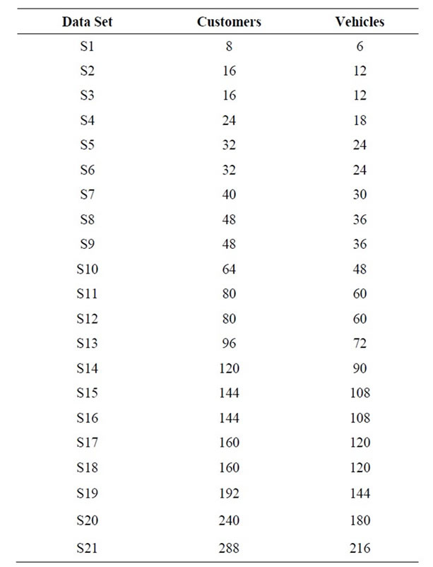
Table 2. Twenty-one data sets from Chen et al. [28].
each of three controls. If the same set of rules is applied for three controls for each vehicle route, then up to 72 different solutions can be created. However, a more diverse set of solutions can be created if a different set of rules for each control is applied for each specific vehicle route within a solution. By randomly selecting which rule to apply for each specific control for each vehicle route, a feasible solution can be generated. Using this approach, 100 solutions with a random application of the rules were generated. These solutions were generated rather quickly, in less than 205 seconds for any particular data set. In order to provide the hybrid genetic algorithm with a strong and diverse start, the initial population for the hybrid genetic algorithm included the 72 combination solutions (directly from the construction heuristic) and the 100 solutions generated by randomly applying the rules for each vehicle route.
3.2. Reproduction Procedures
The 100 randomly generated solutions and the 72 solutions developed by the construction heuristic were used as the initial population. Subsequent offspring populations were created route-by-route using a hybrid genetic algorithm to ensure feasibility. A variety of parameter settings were analyzed and tuned based on the 32 data sets. The results from two fitness approaches are given, shortest route and largest demand unit per distance unit.
3.2.1. Fitness Approach 1: Shortest Route
In order to build a single feasible solution a number of steps must be completed. The current population of solutions provides a set of vehicle routes, and these routes are sorted from shortest to longest based on travel distance. The first fitness approach is to select shorter routes that meet a certain capacity threshold with a greater probability of being selected than longer routes. The shortest feasible route is selected with a probability Pg, and this probability is the same for all solutions and routes. If the vehicle route is selected, then it is added to the current solution and is not included in any further solutions (neither the current solution nor any future solutions) for the current population. If the route is not selected, then the next shortest feasible route is selected with probability Pg. If there are no feasible routes remaining, then the solution is completed using the construction heuristic with a random rule selection for the remaining vehicle routes. By using the construction heuristic, feasibility is ensured. In addition, a number of good solutions from the previous generation are included in the current generation, and bad solutions generated were discarded. This is often referred to as memory [48,49]. This procedure ensures that each generation is better than the previous, and builds a set of good solutions.
The parameters are capacity threshold, probability of route being selected Pg, and the number of solutions from the previous generation kept in the current generation. These parameters were tuned using the 32 data sets. The results of this analysis were to set the capacity threshold as the average vehicle slack (rounded up). The probability, Pg, of a route being selected was set to 20%. The number of solutions kept from the previous generation was set at 10%, which means that the worst 10% of the next generation solutions were discarded (unless they were more favorable than the best 10% from the previous generation). The population size for a generation was set at 100 solutions (except for the initial population which was 172 solutions) and the number of new generations is 20. These values were used to ensure the entire procedure was completed in a timely fashion.
Usually, genetic algorithms incorporate a mutation stage which randomly alters a small portion of the solutions from generation to generation. The SDVRP has side constraints (i.e., capacity, demand) that make mutation difficult while ensuring feasibility. Using the construction heuristic to finish building solutions where no feasible route existed provided a method to alter solutions from generation to generation. This is not a direct mutation, but this method does allow for a portion of the current population to be randomly altered while maintaining feasibility.
The final solution outputted by the hybrid genetic algorithm is the best solution from the last generation. However, it is possible to find this solution in a previous generation, but it would have remained in the current generation since it would have been better than the worst 10% of solutions. This concept goes along with the survival of the fittest goal of genetic algorithms.
3.2.2. Fitness Approach 2: Ratio of Demand Unit Versus Distance Unit
The first fitness approach uses only distances and does not take demand into account during the selection of routes. The second fitness approach sorts the feasible routes based on demand units divided by distance units. The larger this ratio, the more likely the route is selected. The route with the largest demand unit per distance unit is selected with probability Pg. All other parameters remained the same as Fitness Approach 1.
3.2.3. Step-by-Step Procedure for Hybrid Genetic Algorithm
Step 0: Build the initial population using the construction heuristic and 100 random solutions by randomly applying the rules for each of the three controls. The total initial population size is 172.
Step 1: Build the current generation. Sort the routes in the previous population based on the fitness approach. Build a new solution iteratively by route by using Step 2.
Step 2: Select a feasible route with the best fitness value with probability Pg = 0.20. If the feasible route is selected, then add it to the current solution and discard it from being used in later solutions in the current generation. If the feasible route is not selected, then repeat Step 2 (the feasible route is not discarded, but it is not allowed to be selected during the current iteration when selecting a vehicle route).
Step 3: Repeat Step 2 until a complete solution is built or until all feasible routes have been exhausted. If all feasible routes have been exhausted, then use the construction heuristic (by randomly applying the set of rules for each control) to build the remaining routes for the solution.
Step 4: Repeat Steps 2 and 3 until the entire population of 100 solutions is built.
Step 5: Compare the worst 10% of the current population of solutions to the best solutions from the previous generation. Select the best solutions (in terms of shortest travel distance) to remain in the current generation. At most 10 solutions from the current generation will be replaced.
Step 6: Repeat Step 1 until 20 generations are completed.
Step 7: Select the best solution from the final generation. Output as final solution.
4. Computational Experience of the Hybrid Genetic Algorithm
The hybrid genetic algorithm was applied to the data sets from Belenguer et al. [24] and Chen et al. [28] based on the Hybrid Genetic Algorithm Procedures described in Section 3 for both fitness approaches. The procedure was coded in FORTRAN 95 and compiled by GNU FORTRAN on an Intel Xeon Processor 2.49 GHz computer with 8 GB RAM. The best solution was outputted as the final solution.
Section 4.1 describes the performance of the first fitness approach, with the 100 randomly generated solutions and the 72 solutions developed by the construction heuristic as the initial population. Section 4.2 describes performance, with the 100 randomly generated solutions and the 72 solutions developed by the construction heuristic as the initial population, using the second fitness approach.
4.1. Computational Experience Fitness Approach One
Comparative results for 11 data sets from Belenguer et al. [24] are shown in Table 3. The fitness approach one hybrid genetic algorithm time is separated into initial population time and reproduction time, and a total algorithm time is provided. The genetic algorithm produced a solution in the least amount of computer time for each data set (bold), except S51D5. The hybrid genetic algorithm produced the solution with the least amount of travel distance in four cases (bold). Jin et al. [26] found a better solution for three data sets (bold) and Chen et al. [28] in four cases (bold). However, Jin et al. [26] allowed for additional vehicles in their solution, above the minimum number required for the SDVRP, which increases the cost of the overall system.
Comparative results for 21 data sets from Chen et al. [28] are shown in Table 4. The hybrid genetic algorithm produced a solution in the least amount of computer time for each data set (bold), except S20 and S21. The first fitness approach hybrid genetic algorithm found the solution with the least amount of travel distance in 18 cases (bold) Chen et al. [28] found a better feasible solution for three data sets (bold). Both methods found a solution with the same objective for data set S1. Chen et al. [28] reported pseudo lower bounds based on a graphical estimation described in Chen [38]. Chen et al. [28] finds a feasible solution that matches this pseudo lower bound for four instances (italic). The hybrid genetic algorithm finds a feasible solution that matches this pseudo lower bound for five data sets (italic), and finds a feasible solution lower than this bound for ten data sets (italic and
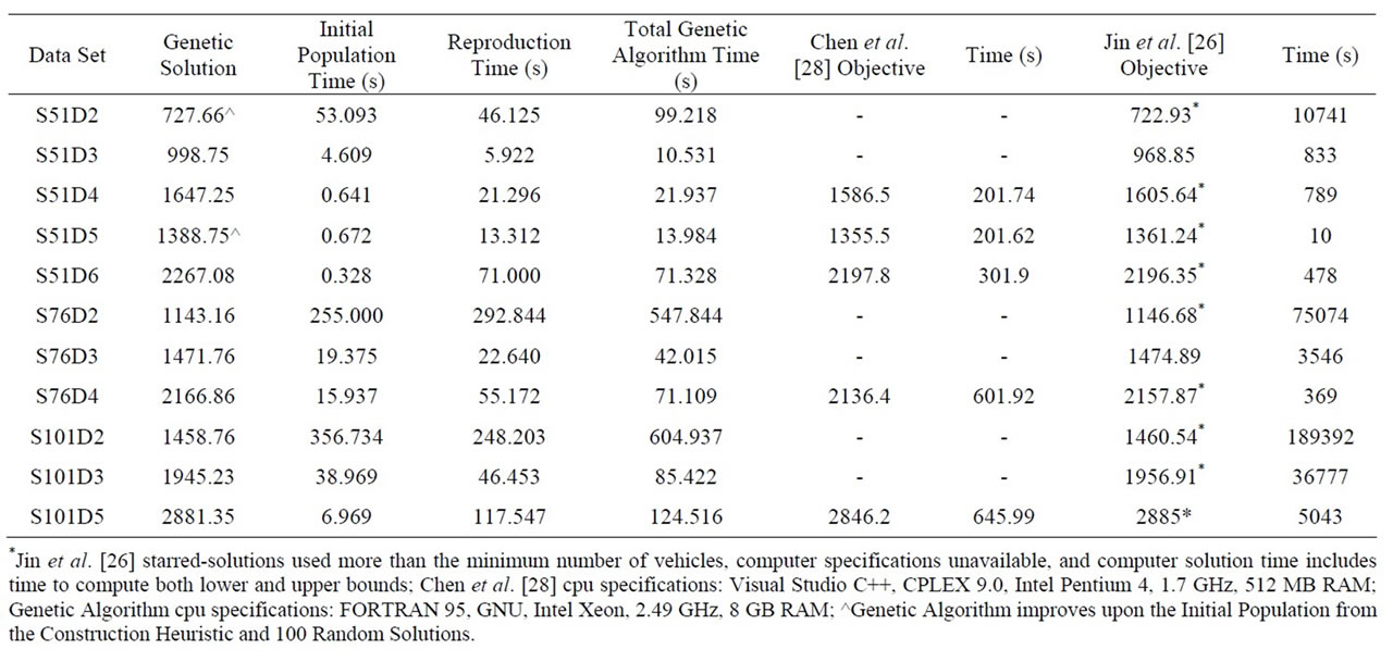
Table 3. Comparing the hybrid genetic algorithm (good start) versus the two-phase method of Chen et al. [28] and the column generation method of Jin et al. [26] for 11 data sets for the first fitness approach.
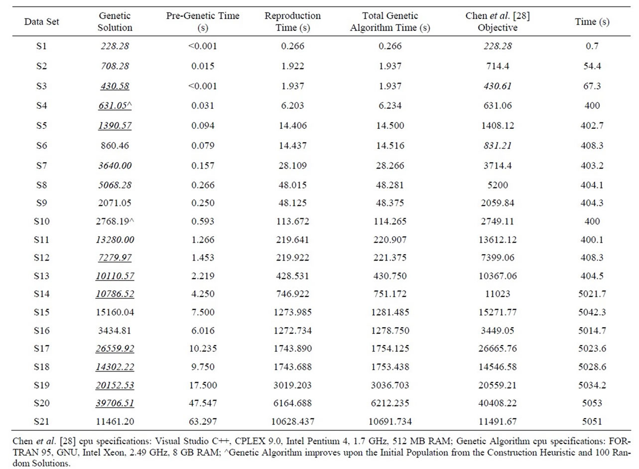
Table 4. Comparing the results of the hybrid genetic algorithm (good start) versus the two-phase method of Chen et al. [28] for 21 data sets for the first fitness approach.
underline).
4.2. Computational Experience Fitness Approach Two
Comparative results for 11 data sets from Belenguer et al. [24] are shown in Table 5. The second fitness approach hybrid genetic algorithm time is separated into initial population time and reproduction time, and a total genetic algorithm time is provided. Both fitness approaches produced the solution with the least amount of travel distance in four cases (bold). Jin et al. [26] found a better solution for three data sets (bold) and Chen et al. [28] in four cases (bold). However, Jin et al. [26] allowed for additional vehicles in their solution, above the minimum number required for the SDVRP, which increases the cost of the overall system.
Comparative results for 21 data sets from Chen et al. [28] are shown in Table 6. The second fitness approach found the solution with the least amount of travel distance in 19 cases (bold). Chen et al. [28] found a better feasible solution for one data set (bold) (i.e., S6). Both methods found a solution with the same objective for data set S1. Chen et al. [28] reported pseudo lower bounds based on a graphical estimation described in Chen [38]. Chen et al. [28] finds a feasible solution that matches this pseudo lower bound for four instances (italic). The hybrid genetic algorithm (both fitness approaches) finds a feasible solution that matches this pseudo lower bound for five data sets (italic), and finds a feasible solution lower than this bound for ten data sets (italic and underline).
4.3. Fitness Approach Comparison
The second fitness approach found a better solution, when compared to the first approach, in six of the 11 data sets from Belenguer et al. [24], they tied in four cases (S76D2, S76D3, S101D2, S101D3), and the first approach found a better solution in only one data set (S51D2). In the four cases in which they tied, these were the four data sets in which the hybrid genetic algorithm outperformed Jin et al. [26] and Chen et al. [28]. For the 21 data sets from Chen et al. [28], when comparing the two fitness approaches, neither is consistently faster than the other in reproduction time. However, the second fitness approach finds a better solution in three cases (S6, S9, S10).
Based on the comparison between the two fitness approaches (with good initial solutions), neither approach seems to be faster than the other. Based on the 32 data sets the two methods were always within 5% of each other in reproduction runtime. However, the second fitness approach provides a better improvement in most cases, with the only exception being S51D2. The two approaches tie in many cases.
5. Summary
This paper focused on solving the SDVRP using a hybrid genetic algorithm. The primary research result of this paper are two fitness approaches for a hybrid genetic algorithm procedure that provide comparable solutions based on objective value and computer time for the SDVRP when compared to a column generation procedure
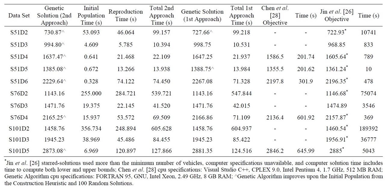
Table 5. Comparing the hybrid genetic algorithm (second fitness approach) versus the two-phase method of Chen et al. [28] and the column generation method of Jin et al. [26] for 11 data sets.
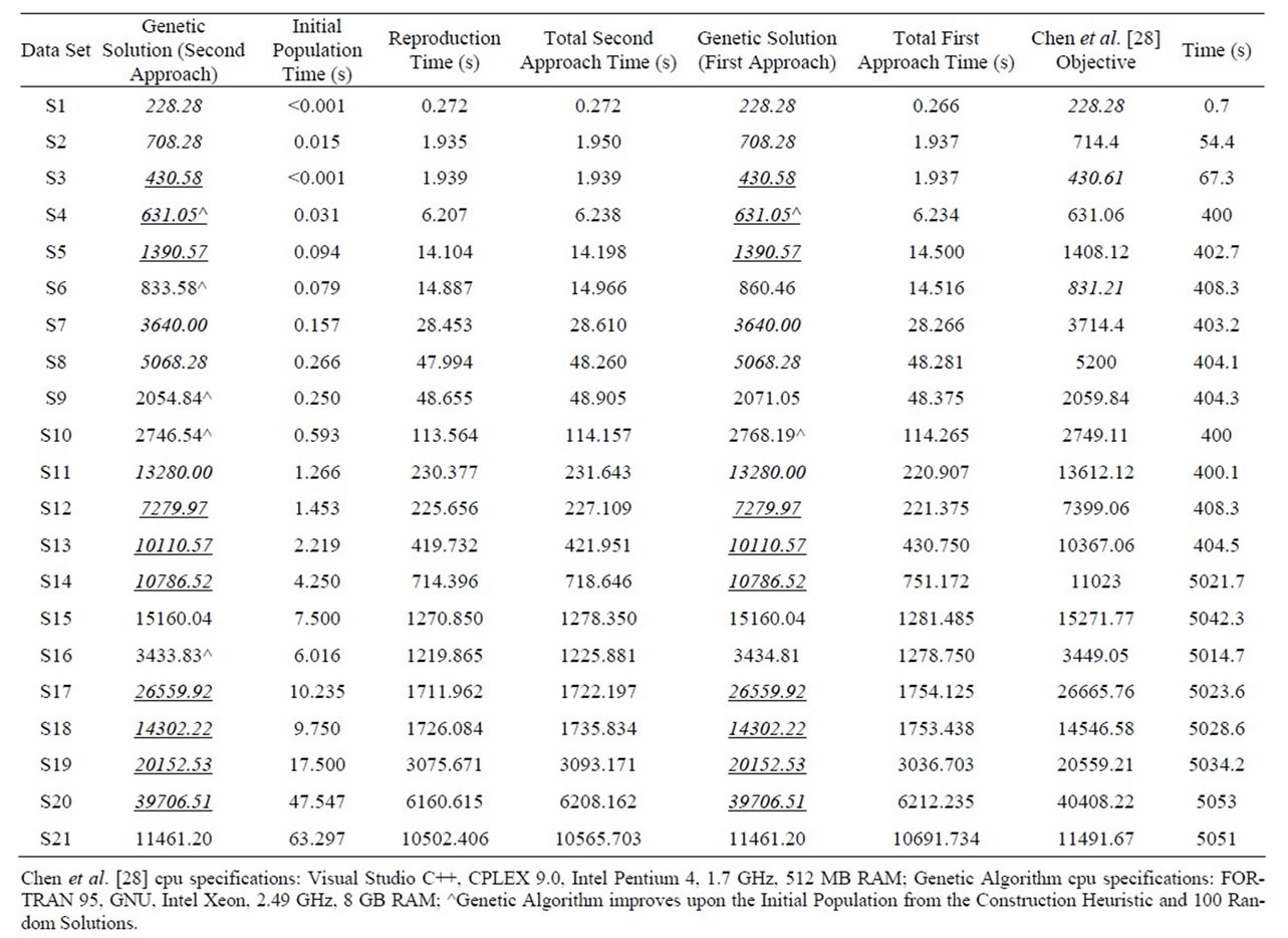
Table 6. Comparing the hybrid genetic algorithm (second fitness approach) versus the two-phase method of Chen et al. [28] for 21 data sets.
[26] and a two-step method [28]. Of the two fitness approaches, the second fitness approach performed better for most of the 32 data sets in terms of solution quality. Neither fitness approach was better than the other in solution time. The hybrid genetic algorithm does not assume symmetric distances, and a future research direction would be to test this heuristic with asymmetric data sets.
REFERENCES
- G. B. Dantzig and J. H. Ramser, “The Truck Dispatching Problem,” Management Science, Vol. 6, No. 1, 1959, pp. 80-91. doi:10.1287/mnsc.6.1.80
- G. Clarke and J. Wright, “Scheduling of Vehicles from a Central Depot to a Number of Delivery Points,” Operations Research, Vol. 12, No. 4, 1964, pp. 568-581. doi:10.1287/opre.12.4.568
- P. Toth and D. Vigo, “Models, Relaxations and Exact Approaches for the Capacitated Vehicle Routing Problem,” Discrete Applied Mathematics, Vol. 123, No. 1-3, 2002, pp. 487-512. doi:10.1016/S0166-218X(01)00351-1
- J. F. Cordeau, M. Gendreau, G. Laporte, J.-Y. Potvin and F. Semet, “A Guide to Vehicle Routing Heuristics,” Journal of the Operational Research Society, Vol. 53, 2002, pp. 512-522. doi:10.1057/palgrave.jors.2601319
- J. F. Cordeau, M. Gendreau, A. Hertz, G. Laporte and J. S. Sormany, “New Heuristics for the Vehicle Routing Problem,” In: A. Langevin and D. Riopel, Eds., Logistics Systems: Design and Optimization, Springer, 2005, pp. 270- 297. doi:10.1007/0-387-24977-X_9
- B. L. Golden and A. A. Assad, “Vehicle Routing: Methods and Studies,” North-Holland, Amsterdam, 1988.
- P. Toth and D. Vigo, “The Vehicle Routing Problem,” Society for Industrial and Applied Mathematics, Philadelphia, 2002.
- G. Laporte and I. H. Osman, “Routing Problems: A Bibliography,” Annals of Operations Research, Vol. 61, No. 1, 1995, pp. 227-262. doi:10.1007/BF02098290
- M. Reimann, “Analysing Risk Orientation in a Stochastic VRP,” European Journal of Industrial Engineering, Vol. 1, No. 2, 2007, pp. 111-130. doi:10.1504/EJIE.2007.014105
- M. Dror and P. Trudeau, “Savings by Split Delivery Routing,” Transportation Science, Vol. 23, No. 2, 1989, pp. 141-145. doi:10.1287/trsc.23.2.141
- M. Dror and P. Trudeau, “Split Delivery Routing,” Naval Research Logistics, Vol. 37, 1990, pp. 383-402.
- M. Affenzeller, S. Winkler, S. Wagner and A. Beham, “Genetic Algorithms and Genetic Programming: Modern Concepts and Practical Applications (Numerical Insights),” Chapman & Hall, 2009. doi:10.1201/9781420011326
- P. Damodaran, N. S. Hirani and M. C. Velez-Gallego, “Scheduling Identical Parallel Batch Processing Machines to Minimise Makespan Using Genetic Algorithms,” European Journal of Industrial Engineering, Vol. 3, No. 2, 2009, pp. 187-206. doi:10.1504/EJIE.2009.023605
- G. B. Alvarenga, G. R. Mateus and G. de Tomi, “A Genetic and Set Partitioning Two-Phase Approach for the Vehicle Routing Problem with Time Windows,” Computers & Operations Research, Vol. 34, No. 6, 2007, pp. 1561-1584. doi:10.1016/j.cor.2005.07.025
- X. Wang, B. L. Golden and E. A. Wasil, “Using a Genetic Algorithm to Solve the Generalized Orienteering Problem,” In: B. Golden, S. Raghavan and E. Wasil, Eds., The Vehicle Routing Problem: Latest Advances and New Challenges, Springer, 2008, pp. 263-274. doi:10.1007/978-0-387-77778-8_12
- M. Dror, G. Laporte and P. Trudeau, “Vehicle Routing with Split Deliveries,” Discrete Applied Mathematics, Vol. 50, No. 3, 1994, pp. 239-254. doi:10.1016/0166-218X(92)00172-I
- P. W. Frizzell and J. W. Giffin, “The Split Delivery Vehicle Scheduling Problem With Time Windows and Grid Network Distances,” Computers and Operations Research, Vol. 22, No. 6, 1995, pp. 655-667. doi:10.1016/0305-0548(94)00040-F
- P. W. Frizzell and J. W. Giffin, “The Bounded Split Delivery Vehicle Routing Problem with Grid Network Distances,” Asia Pacific Journal of Operational Research, Vol. 9, 1992, pp. 101-116.
- C. Archetti, M. Savelsbergh and A. Hertz, “A Tabu Search Algorithm for the Split Delivery Vehicle Routing Problem,” Transportation Science, Vol. 40, No. 1, 2006, pp. 64-73. doi:10.1287/trsc.1040.0103
- R. E. Aleman and R. R. Hill, “A Tabu Search with Vocabulary Building Approach for the Vehicle Routing Problem with Split Demands,” International Journal of Metaheuristics, Vol. 1, No. 1, 2010, pp. 55-80.
- C. Archetti, M. Savelsbergh and M. G. Speranza, “Worst-Case Analysis for Split Delivery Vehicle Routing Problems,” Transportation Science, Vol. 40, No. 2, 2006, pp. 226-234. doi:10.1287/trsc.1050.0117
- C. Archetti, M. Savelsbergh and M. G. Speranza, “To Split or Not to Split: That Is the Question,” Transportation Research Part E, Vol. 44, No. 1, 2008, pp. 114-123. doi:10.1016/j.tre.2006.04.003
- C. Lee, M. A. Epelman, C. C. White and Y. A. Bozer, “A Shortest Path Approach to the Multiple-Vehicle Routing Problem with Split Pick-Ups” Transportation Research Part B, Vol. 40, No. 4, 2006, pp. 265-284. doi:10.1016/j.trb.2004.11.004
- J. M. Belenguer, M. C. Martinez and E. A. Mota, “Lower Bound for the Split Delivery VRP,” Operations Research, Vol. 48, No. 5, 2000, pp. 801-810. doi:10.1287/opre.48.5.801.12407
- M. Jin, K. Liu and R. O. Bowden, “A Two-Stage Algorithm with Valid Inequalities for the Split Delivery Vehicle Routing Problem,” International Journal of Production Economics, Vol. 105, No. 1, 2007, pp. 228-242. doi:10.1016/j.ijpe.2006.04.014
- M. Jin, K. Liu and B. Eksioglu, “A Column Generation Algorithm for the Vehicle Routing Problem with Split Delivery,” Proceedings of the 2007 Industrial Engineering Research Conference, Nashville, 19-23 May 2007.
- M. Jin, K. Liu and B. Eksioglu, “A Column Generation Approach for the Split Delivery Vehicle Routing Problem,” Operations Research Letters, Vol. 36, No. 2, 2008, pp. 265-270. doi:10.1016/j.orl.2007.05.012
- S. Chen, B. Golden and E. Wasil, “The Split Delivery Vehicle Routing Problem: Applications, Test Problems, and Computational Results,” Networks, Vol. 49, No. 4, 2007, pp. 318-329. doi:10.1002/net.20181
- W. Burrows, “The Vehicle Routing Problem with Loadsplitting: A Heuristic Approach,” 24th Annual Conference of the Operational Research Society of New Zealand, Auckland, 18-19 August 1988, pp. 33-38.
- J. H. Wilck IV and T. M. Cavalier, “A Construction Heuristic for the Split Delivery Vehicle Routing Problem,” American Journal of Operations Research, 2012, in press.
- R. E. Aleman, X. Zhang and R. R. Hill, “An Adaptive Memory Algorithm for the Split Delivery Routing Problem,” Journal of Heuristics, 2008, Available Online.
- C. Archetti and M. G. Speranza, “The Split Delivery Vehicle Routing Problem: A Survey. The Vehicle Routing Problem: Latest Advances and New Challenges,” Operations Research/Computer Science Interfaces Series, Vol. 43, Part I, 2008, pp. 103-122. doi:10.1007/978-0-387-77778-8_5
- D. J. Gulczynski, B. Golden and E. Wasil, “Recent Developments in Modeling and Solving the Split Delivery Vehicle Routing Problem,” Tutorials in Operations Research, INFORMS, 2008, pp. 170-180.
- R. E. Aleman, “A Guided Neighborhood Search Applied to the Split Delivery Vehicle Routing Problem,” Dissertation Thesis, Wright State University, 2009.
- J. H. Wilck IV, “Solving the Split Delivery Vehicle Routing Problem,” Dissertation Thesis, Pennsylvania State University, 2009.
- K. Liu, “A Study on the Split Delivery Vehicle Routing Problem,” Dissertation Thesis, Mississippi State University, 2005.
- M. A. Nowak, “The Pickup and Delivery Problem with Split Loads,” Dissertation Thesis, Georgia Institute of Technology, 2005.
- S. Chen, “A Study of Four Network Problems in Transportation, Telecommunications, and Supply Chain Management,” Dissertation Thesis, University of Maryland, 2007.
- P. Mullaseril, M. Dror and J. Leung, “Split-Delivery Routing Heuristics in Livestock Feed Distribution,” Journal of the Operational Research Society, Vol. 48, 1997, pp. 107-116.
- G. Sierksma and G. A. Tijssen, “Routing Helicopters for Crew Exchanges on Off-Shore Locations,” Annals of Operations Research, Vol. 76, 1998, pp. 261-286. doi:10.1023/A:1018900705946
- S. Song, K. Lee and G. Kim, “A Practical Approach to Solving a Newspaper Logistics Problem Using a Digital Map,” Computers and Industrial Engineering, Vol. 43, No. 1-2, 2002, pp. 315-330. doi:10.1016/S0360-8352(02)00077-3
- D. Goldberg, “Genetic Algorithms in Search Optimization and Machine Learning,” Addison Wesley, Reading, 1989.
- W. L. Winston and M. Venkataramanan, “Introduction to Mathematical Programming, Operations Research: Volume One,” 4th Edition, Thomson Learning, 2003.
- M. Gendreau, G. Laporte and J.-Y. Potvin, “Vehicle Routing: Modern Heuristics,” In: E. Aarts and J. K. Lenstra, Eds., Local Search in Combinatorial Optimization, John Wiley & Sons, Inc., New York, 1997, pp. 323-330.
- M. Gendreau, G. Laporte and J.-Y. Potvin, “Metaheuristics for the Capacitated VRP,” In: P. Toth and D. Vigo, Eds., The Vehicle Routing Problem, Society for Industrial and Applied Mathematics, Philadelphia, 2002, pp. 140- 144.
- B. M. Baker and M. A. Ayechew, “A Genetic Algorithm for the Vehicle Routing Problem,” Computers & Operations Research, Vol. 30, No. 5, 2003, pp. 787-800. doi:10.1016/S0305-0548(02)00051-5
- G. Jeon, H. R. Leep and J. Y. Shim, “A Vehicle Routing Problem Solved by Using a Hybrid Genetic Algorithm,” Computers & Industrial Engineering, Vol. 53, No. 4, 2007, pp. 680-692. doi:10.1016/j.cie.2007.06.031
- S. J. Louis and G. Li, “Augmenting Genetic Algorithms with Memory to Solve Traveling Salesman Problems,” Proceedings of the Joint Conference on Information Sciences, 1997.
- A. Acan and Y. Tekol, “Chromosome Reuse in Genetic Algorithms,” Lecture Notes in Computer Science, GECCO 2003, LNCS 2723, Springer-Verlag, Berlin, 2003, pp. 695-705.