 Applied Mathematics, 2011, 2, 1225-1235 doi:10.4236/am.2011.210171 Published Online October 2011 (http://www.SciRP.org/journal/am) Copyright © 2011 SciRes. AM Generalization of Certain Subclasses of Multivalent Functions with Negative Coefficients Defined by Cho-Kwon-Srivastava Operator Elsayed A. Elrifai, Hanan E. Darwish, Abdusalam R. Ahmed Department of Mathematics, Faculty of Science, University of Mansoura, Mansoura, Egypt E-mail: Rifai@mans.edu.eg, Darwish333@yahoo.com, Abdusalam5056@yahoo.com Received November 1, 2010; revised July 6, 2011; accepted July 13, 2011 Abstract Making use of the Cho-Kwon-Srivastava operator, we introduce and study a certain SCn (j, p, λ, α, δ) of p-valently analytic functions with negative coefficients. In this paper, we obtain coefficient estimates, distor- tion theorem, radii of close-to-convexity, starlikeness, convexity and modified Hadamard products of func- tions belonging to the class SCn (j, p, λ, α, δ). Finally, several applications investigate an integral operator, and certain fractional calculus operators also considered. Keywords: Multivalent Functions, Cho-Kwon-Srivastava Operator, Modified-Hadamard Product, Fractional Calculus 1. Introduction Let denote the class of functions of the form: ,Tjp 0; ,1,2,3,, pk kk kjp fzzazapj N (1.1) which are analytic and p-valent in the open unit disc :1 Uzz. A function , zTjp is said to be p-valently starlike of order if it satisfies the inequal- ity : Re;0; . zf zzUpp N fz (1.2) We denote by , j Tp the class of all p-valently starlike functions of order . Also a function z is said to be p-valently convex of order ,Tjp if it satisfies the inequality: Re1; 0;. zf zzUpp N fz (1.3) We denote by , j Cp ,, 0;. jj zf z fzC pTp p pp N (1.4) The classes , j Tp and , j Cp are studied by Owa [3]. In [4] Wang et al. defined Cho-kwon-Srivastava op- erator which ,,:, , pj acfzTjpTjp , by ,,! kp kp k pj k kjp kp pc ac fzzaz kpa (1.5) for 0 ,0,1,2,3, ,,acRZz Up and 1; 11; k k kk 0 .N Clearly, ,1 , pac is the well-known Cho-kwon- Srivastava operator (see [5]) where the class of all p-valently convex functions of order . We note that (see for ex- ample Duren [1] and Goodman [2]) 11 ,, 1,1,,1, pj pj zf z pfzp p  E. A. ELRIFAI ET AL. 1226 and 1 ,1 ,, p paaDf zp where is the well-known Ruscheweyh deriva- tive of -th order. 1p D p 1 With the help of the Cho-Kwon-Srivastava ,,ac fz , pj we say that a function z belonging to is in the class ,Tjp ,,,,j p n SC if and only if 2 ,, ,, 0 ,, Re 1, , , pj pj pj pj zacfzz acfz ac fzzac fz pNjN (1.6) We note that: 1) when 0, we have , , , Re , pj pj zacfz ac fz which is the class of starlike of order . 2) when 0 , , 1ap 1 , , we have the class 1c Re; 0 zf zp fz which is the class of starlike functions of order stu- died by Owa [3] and Y amakawa [6] 3) when 1, we have , , , Re 1; , 0 pj pj zacfz ac fz p which is the class of convex operator of order . 4) when 1 , 1ap , , 1c1 , we have Re 1;0 zf zp fz which is the class of convex functions of order stud- ied by Owa [3] and Yam akawa [6]. In our present paper, we shall make use of the familiar ,cp defined by (c.f. [7,8], see also [9]) 1 ,0d, z c cp c cp fz tftt z (1.7) ,; , zTjpcppN, as well as the fractional calculus operator D for which it is well known that (see, for details, [10,11]; see also Section 5 below) 1, 1 1; z Dz z R (1.8) in terms of Gamma functions. 2. Coefficient Estimates Theorem 1. Let the function z defined by (1.1). Then ,,,, n fzSC jp if and only if 11 ! 11 kp kp k kjp kp pc kk kpa pp a (2.1) 0 ;0,01, ,,.zUppjNnN Proof. Assume that the inequality (2.1) holds true. Then we have 11 ! 11 1 ! kp kp k kjpkp kp kp k kjpkp pc jpk a kpa pc kkapp kpa 1 that is, that 11 11 ! kp kp k kjp kp pc pp ka kpa jp . Since Copyright © 2011 SciRes. AM  E. A. ELRIFAI ET AL. 1227 11 11 ! 11 11 ! 11 11 11 ! kp kpkp k kjpkp kp kp kp k kjp kp kp kp k kjp kp pc pkaz kpa pc pkaz kpa pc jp pka kpa jp 0. Then we find that 2 ,, ,, ,, 1, , 11 ! 11 11 ! 11 ! 1 pj pj pj pj kp kp kp k kjp kp kp kp kp k kjpkp kp kp k kjpkp zacfzzacfzp acf zzacf z pckpk az kpa pc kk kpa pckpk a kpa p az . 111 ! kp kp k kjp kp p pc ka kpa (2.2) This shows that the values of the function 2 ,, ,, ,, 1, , pj pj pj pj zacfzz acfz z ac fzzac fz (2.3) lie in a circle which is centered at and whose radius is wp .p Hence z satisfies the condition (1.6). Conversely, assume that the function z is in the class ,,,, n SCj p . Then we have 2 ,, ,, ,, Re 1, , 11 11 ! Re 11 11 ! pj pj pj pj kp kpkp k kjp kp kp kpkp k kjpkp zacfzz acfz ac fzzac fz pc pp kkaz kpa pc pk kpa az (2.4) for some some , p, 0,p 01 jN , 0, and Choose values of z on the real axis so that given by (2.3) is real. Upon clearing the denominator in (2.4) and letting through real values, we can see that nN.zU z 1z 11 11 ! 11 11 ! kp kp k kjpkp kp kp k kjpkp pc pp kka kpa pc pk kpa . a (2.5) Copyright © 2011 SciRes. AM  E. A. ELRIFAI ET AL. Copyright © 2011 SciRes. AM 1228 Thus we have the inequality (2.1). Corollary 1. Let the function z defined by (1.1) be in the class ,,,, n SCj p . Then 11 1 ! ,, . k kp kp kp pp apckk kpa kjppjN 1 (2.6) The result is sharp for the function z given by 0 11 11 ! ,, ,. k kp kp kp pp zz z pckk kpa kjppjNnN (2.7) 3. Distortion Theorem Theorem 2. If a function z defined by (1.1) is in the class ,,,, n SCj p then 11 ! ! !11 ! ! 11 ! ! !11 ! ! jpm jj j pm m jj j ppjp pzz pc pm jpjp jpm ja ppjp p fzz z pc pm jpjp jpm ja (3.1) 0 ;0;01,,,.zUppj NnN The result is sharp for the function z given by 0 11 ., ,. 11 ! pj jj j pp fzzzpj Nn N pc jp jp ja p (3.2) Proof. In view of Theorem 1, we have 11 11 !! !1 11 !11 jj kp kp jkp k k kjpkjp pc pc jp jpkk ja kpa ka a ppjp pp which readily yields 11 ! !. 11 ! k kjp jj j ppjp ka pc jp jp ja (3.3) Now, by differentiating both sides of (1.1) m times, we obtain !! !! ,, . m m k kjp pk km zz a pm km kjpjpN z (3.4) Theorem 2, follows from (3.3) and (3.4). Finally, it is easy to see that the bou nds in (3.1) are at- tained for the function z given by (3.2). 4. Radii of Close-to-Convexity, Starlikeness and Convexity Theorem 3. Let the function zdefined by (1.1) be in the class ,,,, n SCj p then 1) z is p-valently close-to-convex of order 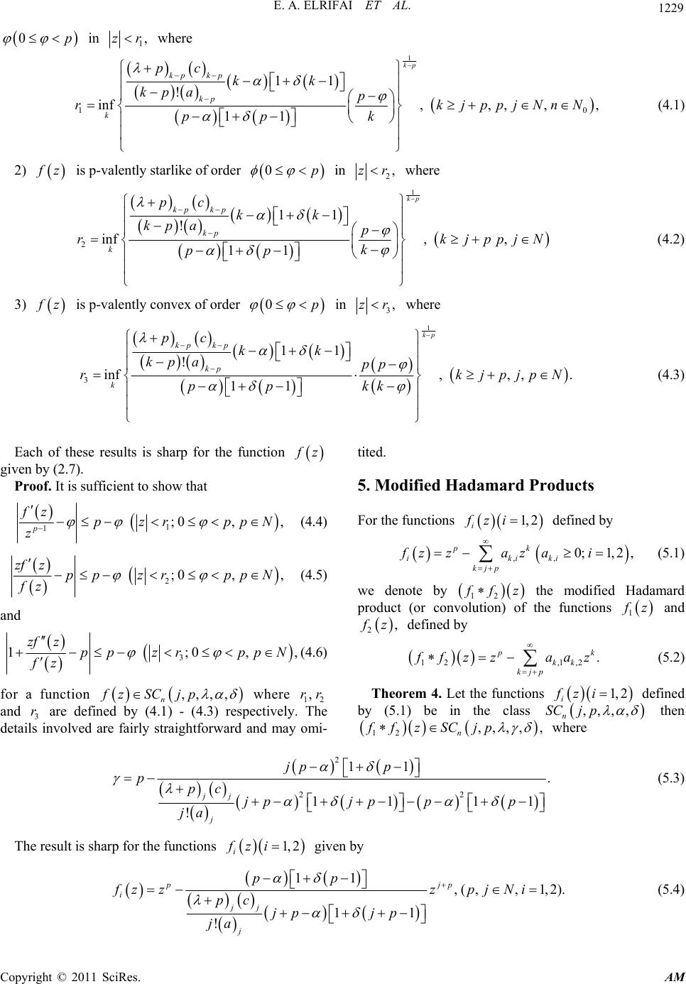 E. A. ELRIFAI ET AL. 1229 0p in 1,zr where 1 1 0 11 ! inf,, ,,, 11 kp kp kp kp k pckk kpa p rk k pp jppjNnN (4.1) 2) z is p-valently starlike of order in 0p 2,zr where 1 2 11 ! inf,, 11 kp kp kp kp k pckk kpa p rk k pp jppjN (4.2) 3) z is p-valently convex of order in 0p 3,zr where 1 3 11 ! inf,,,. 11 kp kp kp kp k pckk kpa pp rk kk pp jpjpN (4.3) Each of these results is sharp for the function z given by (2. 7) . Proof. It is sufficient to show that 1 1;0, , p fz pzr ppN z (4.4) 2;0, , zf zppzrppN fz (4.5) and 3 1;0 zf zppzrppN fz ,, (4.6) for a function ,,,, n fzSC jp where 12 and 3 are defined by (4.1) - (4.3) respectively. The details involved are fairly straightforward and may omi- ,rr r tited. 5. Modified Hadamard Products For the func tions 1, 2 i fzi defined by ,, 0;1,2 , pk ikiki kjp fzzaz ai (5.1) we denote by 12 fz the modified Hadamard product (or convolution) of the functions 1 z and 2, z defined by 12 ,1,2 . k kk kjp fzz aaz (5.2) Theorem 4. Let the functions defined by (5.1) be in the class 1, 2 i fzi ,,,, n SCj p then 12 ,,,, n ffz SCjp, where 2 22 11 . 11 1 ! jj j jp p ppc jpjp pp ja 1 (5.3) The result is sharp for the functions given by 1, 2 i fzi 11 ,(,,1,2). 11 ! pj i jj j pp fzzzpjNi pc jp jp ja p (5.4) Copyright © 2011 SciRes. AM 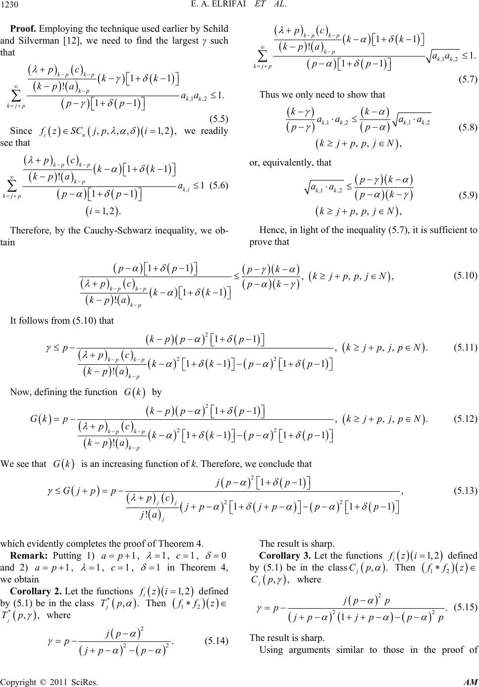 E. A. ELRIFAI ET AL. Copyright © 2011 SciRes. AM 1230 Proof. Employing the technique used earlier by Schild and Silverman [12], we need to find the largest γ such that ,1 ,2 11 !1. 11 kp kp kp kk kjp pckk kpa aa pp (5.5) Since we readily see that ,,,, 1,2, in fzSC jpi , 11 !1 11 1, 2. kp kp kp ki kjp pckk kpa a pp i (5.6) Therefore, by the Cauchy-Schwarz inequality, we ob- tain ,1 ,2 11 !1. 11 kpkp kp kk kjp pc kk kpa aa pp (5.7) Thus we onl y need to show that ,1 ,2,1 ,2 ,, , kk kk kk aa aa pp kjppjN (5.8) or, equivalently, that ,1 ,2 ,, , kk pk aa pk kjppjN (5.9) Hence, in light of the inequality (5.7), it is sufficient to prove that 11 ,,, 11 ! kp kp kp pp pk kjppjN pc pk kk kpa , (5.10) It follows fro m (5.10) that 2 22 11 ,,, 11 11 ! kp kp kp kppp pk pckkpp kpa .jpjpN (5.11) Now, defining the function Gk by 2 22 11 ,,, 11 11 ! kp kp kp kppp Gkpkjp jpN pckkpp kpa . (5.12) We see that is an increasing function of k. Ther efore, we con clude that Gk 2 22 11 , 11 ! jj j jp p Gj pppc jpjp pp ja 1 (5.13) which eviden tly completes the proof of Theorem 4. Remark: Putting 1) , 1ap 1 , , 1c0 and 2) , 1ap 1 , 1c , 1 in Theorem 4, we obtain Corolla ry 2. Let the functions defined by (5.1) be in the class 1, 2 i fzi . *, j Tp Then 12 fz *,, j Tp where 2 22 . jp p jp p (5.14) The result is sharp. Corollary 3. Let the functions defined by (5.1) be in the class. 1, 2 i fzi , j Cp Then 12 fz ,, j Cp where 2 22 . 1 jp p p jpjppp (5.15) The result is sharp. Using arguments similar to those in the proof of  E. A. ELRIFAI ET AL. 1231 Theorem 4, we obtain the following result. Theorem 5. Let the function 1 z defined by (5.1) be in the class ,,,, n SCj p Suppose also that the function 2 z defined by (5.1) be in the class ,,,,SCj p n , Then 12 ,,,, n ff z SCjp, where 11 , 11 ! kp kp kp jp pp ppcjpjpjp kpa (5.16) and 11pp p . (5.17) The result is the best possible for the functions 1 11 ,, 11 ! pj jj j pp fzzzpj N pc jp jp ja p (5.18) and 2 11 ,, 11 ! pj jj j pp fz zzpjN pc jpjp ja . p (5.19) Theorem 6. Let the functions 1, 2,, i zi m ,,,, nj p defined by (5.1) be in the class SC . Then the function 2, 1, p ki kjpi hz za z k (5.20) belongs to the class ,,,, n SCj p where 2 22 11 . 11 1 ! jj j jm pp ppc jpjp mpp ja 1 (5.21) The result is sharp for the functions 1, 2,, i zi m given by (5.4). Proof. Noting that 2 2 2, , 11 11 !! 1, 11 11 ,,,,1,2, , kp kpkp kp kp kp ki ki kjp kjp in pc pc kk kk kpa kpa aa pp pp fzSC jpim (5.22) we have 2 2, 1 11 ! 11. 11 kp kp m kp ki kjp i pckk kpa a mpp (5.23) Therefore, we have find largest such that Copyright © 2011 SciRes. AM 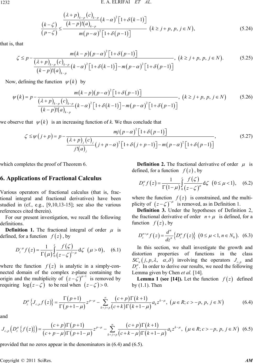 1232 E. A. ELRIFAI ET AL. 2 2 11 !,, , 11 kp kp kp pckk kpa kkjppjN pmpp (5.24) that is, that 2 22 11 ,,, 11 11 ! kp kp kp mkp pp pk pckkmpp kpa .jppjN (5.25) Now, defining the function by k 2 22 11 ,,, 11 11 ! kp kp kp mkp pp kp kjppjN pckkmpp kpa (5.26) we observe that is an increasing function of k. We thus conclude that k 2 22 11 , 11 1 ! jj j mj pp jp ppc jpjp mpp ja 1 (5.27) which completes the proo f of Theorem 6. 6. Applications of Fractional Calculus Various operators of fractional calculus (that is, frac- tional integral and fractional derivatives) have been studied in (cf., e.g., [9,10,13-15]; see also the various references cited therein). For our present investigation, we recall the following definitions. Definition 1. The fractional integral of order is defined, for a function z, by 1 0 1d z z f Dfz z 0 , (6.1) where the function z is analytic in a simply-con- nected domain of the complex z-plane containing the origin and the multiplicity of 1 z is removed by requiring log z to be real when 0. z Definition 2. The fractional derivative of order is defined, for a function z, by 0 1d01 1 , z f Dfz z z (6.2) where the function z is constrained, and the multi- plicity of z is r emoved, as in D efinition 1. Definition 3. Under the hypotheses of Definition 2, the fractional derivative of order n is defined, for a function z, by 0 01, n n zz n d Dfz DfznN dz . (6.3) In this section, we shall investigate the growth and distortion properties of functions in the class ,,, n SCj p , involving the operators ,cp and . D In order to derive our results, we need the following Lemma given by Chen et al. [14]. Lemma 1 (see [14]). Let the function z defined by (1.1). Then , 11 ,;,, 11 pk zcp k kjp pcpk DJfzzazRc ppjN pckk (6.4) and , 11 ,;,, 11 pk cp zk kjp cppcp k DfzzazRc ppjN cppckk (6.5) provided that no zeros appear in the denominators in (6.4) and (6.5). Copyright © 2011 SciRes. AM  E. A. ELRIFAI ET AL. 1233 Theorem 7. Let the function z defined by (1.1) be in the class ,,,, n SCj p . Then , 111 1, 1111 ! ;0;01;0;,, jp zcp jj j cp jppp p DJfzzz pc pcjp jpjpjp ja zUpcppjN (6.6) and , 111 1, 1111 ! ;0;01;0;,,. jp zcp jj j cp jppp p DJfzzz pc pcjp jpjpjp ja zUpcppj N (6.7) Each of the assertion (6.6) and (6.7) is sharp. Proof. In view of Theorem 1, we have 11 11 !! 1, 11 11 jj kp kp jkp k k kjpkjp pcp c jpjpjp k jakpa aa pp pp (6.8) which readily yields 11 . 11 ! k kjpjj j pp apc jp jp ja (6.9) Consider the function z defined in U by , 11 11 , 1 1 k zcp k kjp pk k kjp pcpkp zzDJfzz pckk zkazzU az p where 11 ,,, 0. 11 cp kp kkjp ck kp pjN (6.10) Since is a decreasing function of k when k 0 , we get 11 0, 11 cp jpp kjp cppjN cjp jpp ,,0. (6.11) Thus, by using (6. 9) an d (6 .1 1), we deduce that 111 1, 1111 ! pjp k kjp jp jj j Fzzj pza cp jpppp z z pc cjp jppjpjp ja Copyright © 2011 SciRes. AM  E. A. ELRIFAI ET AL. Copyright © 2011 SciRes. AM 1234 and 111 1, 1111 ! pjp k kjp jp jj j Fzzj pza cp jpppp z z pc cjp jppjpjp ja which yield the inequ alities (6.6 ) and (6 .7 ) of Theorem 7. The equalities in (6.6) and (6.7) are attained for the func-tion z given by , 11 1 1 111 ! jp zcp jj j cppjpp p DJfzzz pc pcjpjpjpjp ja 1 (6.12) or, equivalently, by , 11 . 11 !1 jp cp jj j cppp Jfz zz pc cjp jpjpjp ja (6.13) Theorem 8. Let the function z defined by (1.1) be in the class .,,,, n SCj p Then Thus we complete the proof of Theorem 7. Using arguments similar to those in the proof of Theorem 7, we obtain the following result. , 111 1, 1111 ! ;0,01,01,, ,, jp zcp jj j cp jppp p DJfzzz pc pcjpjpjpjp ja zUpcpjp N (6.14) and , 111 1, 1111 ! ;0,01,01, ,. jp zcp jj j cp jppp p DJfzzz pc pcjpjpjpjp ja zUpjp N (6.15) Each of the assertions (6.14) and (6.15) is sharp. 7. References [1] P. L. Duren, “Univalent functions,” In: Grundlehen der Mathematischen Wissenschaften, Vol. 259, Springer- Verlag, New York, 1983. [2] A. W. Goodman, “Univalent Functions, Vols. I and II,” Polygonal Publishing House, Washington, 1983. [3] S. Owa, “The Quasi-Hadamard Products of Certain Ana-  E. A. ELRIFAI ET AL. 1235 lytic Functions,” In: H. M. Srivastava and S. Owa, Eds., Current Topics in Analytic Function Theory, World Sci- entific Publishing Company, Singapore, 1992, pp. 234- 251. [4] Z.-G. Wang, R. Aghalary, M. Darus and R. W. Ibrahim, “Some Properties of Certain Multivalent Analytic Func- tions Involving the Cho-Kwon-Srivastava Operator,” Journal of Mathematical and Computer Modelling, Vol. 49, No. 9-10, 2009, pp. 1969-1984. [5] N. E. Cho, O. S. Kwon and H. M. Srivastava, “Inclusion Relationships and Argument Properties for Certain Sub- classes of Multivalent Functions Associated with a Fam- ily of Linear Operators,” Journal of Mathematical Analy- sis and Applications, Vol. 292, No. 2, 2004, pp. 470-483. doi:10.1016/j.jmaa.2003.12.026 [6] R. Yamakawa, “Certain Subclasses of p-Valently Starlike Functions with Negative Coefficients,” In: H. M. Srivas- tava and S. Owa, Eds., Current Topics in Analytic Func- tion Theory, World Scientific Publishing Company, Sin- gapore, 1992, pp. 393-402. [7] S. D. Bernardi, “Convex and Starlike Univalent Func- tions,” Transactions of the American Mathematical Soci- ety, Vol. 135, 1969, pp. 429-446. doi:10.1090/S0002-9947-1969-0232920-2 [8] A. E. Livingston, “On the Radius of Univalence of Cer- tain Analytic Functions,” Proceedings of the American Mathematical Society, Vol. 17, No. 2, 1966, pp. 352-357. doi:10.1090/S0002-9939-1966-0188423-X [9] H. M. Srivastava and S. Owa (Eds.), “Current Topics in Analytic Function Theory,” World Scientific Publishing Company, Singapore, 1992. [10] S. Owa, “On Distortion Theorems. I,” Kyungpook Ma- thematical Journal, Vol. 18, 1978, pp. 55-59. [11] H. M. Srivastava and M. K. Aouf, “A Certain Fractional Derivative Operator and Its Applications to a New Class of Analytic and Multivalent Functions with Negative Co- efficients. I and II,” Journal of Mathematical Analysis and Applications, Vol. 171, No. 1, 1992, pp. 1-13. doi:10.1006/jmaa.1995.1197 [12] A. Schild and H. Silverman, “Convolutions of Univalent Functions with Negative Coefficients,” Annales Univer- sitatis Mariae Curie-Sklodowska Section A, Vol. 29, 1975, pp. 99-107. [13] O. Altintas, H. Irmak and H. M. Srivastava, “Fractional Calculus and Certain Starlike Functions with Negative Coefficients,” Computers and Mathematics with Applica- tions, Vol. 30, No. 2, 1995, pp. 9-15. doi:10.1016/0898-1221(95)00073-8 [14] M.-P. Chen, H. Irmak and H. M. Srivastava, “Some Fam- ilies of Multivalently Analytic Functions with Negative Coefficients,” Journal of Mathematical Analysis and Ap- plications, Vol. 214, No. 2, 1997, pp. 674-690. doi:10.1006/jmaa.1997.5615 [15] H. M. Srivastava and S. Owa (Eds.), “Univalent Func- tions, Fractional Calculus, and Their Applications,” Ellis Horwood Limited, Chichester, 1989. Copyright © 2011 SciRes. AM
|