American Journal of Oper ations Research, 2011, 1, 147-154
doi:10.4236/ajor.2011.13016 Published Online September 2011 (http://www.SciRP.org/journal/ajor)
Allocation of Repairable and Replaceable Components
for a System Availability Using Selective Maintenance
with Probabilistic Maintenance Time Constraints
Irfan Ali1*, Mohammed Faisal Khan2, Yashpal Singh Raghav1, Abdul Bari1
1Department of Statistics & Operations Research, Aligarh Muslim University, Aligarh, India
2Department of Mat hem at i cs, Integral University, Lucknow, India
Received April 23, 2011; revised May 19, 2011; accepted June 8, 2011
Abstract
In this paper, we obtain optimum allocation of replaceable and repairable components in a system design.
When repair and replace time are considered as random in the constraints. We convert probabilistic con-
straint into an equivalent deterministic constraint by using chance constrained programming. We have used
the selective maintenance policy to determine how many components to be replaced & repaired within the
limited maintenance time interval and cost. A Numerical example is presented to illustrate the computational
procedure and problem is solved by using LINGO Software.
Keywords: Selective Maintenance, Availability, Optimization and Allocation, Chance Constraints
1. Introduction
In many industrial environments, systems are required to
perform a sequence of operations (or missions) with fi-
nite breaks between each operation. During these breaks,
it may be advantageous to perform repair and replace-
ment on some of the system components. However, it
may be impossible to perform all desirable maintenance
activities prior to the beginning of the next mission due
to limitations on maintenance resources. In this paper,
we have consider that the maintenance (i.e. repair and
replace) time in general are unknown (are of random
character). For this a mathematical programming frame-
work is established for assisting decision-makers in de-
termining the optimal subset of maintenance activities to
perform prior to beginning of the next mission. This de-
cision-making process is referred to as selective mainte-
nance. The selective maintenance models presented al-
low the decision-maker to consider limitations on main-
tenance time and budget, as well as the reliability of the
system. Selective maintenance is an open research area
that is consistent with the modern industrial objective of
performing more intelligent and efficient maintenance.
Rice et al. [1] define a Mathematical programming
Model for solving selective maintenance problem. Cas-
sady et al. [2] extend the mathematical programming
model problem by permitting subsystems to be com-
prised of non identical components in any structure,
adding a second resource constraint (representing main-
tenance cost), and creating two additional selective
maintenance formulations that minimize resource con-
sumption as the objective function and include mission
reliability as a constraint. Cassady et al. [3] extend
mathematical programming model problem in two ways.
First the life distributions of system components are
specified to be weibull distributions. Second, the decision
maker is given multiple maintenance options: minimal
repair on failed components, replacement of failed com-
ponents and replacement of functioning components
(preventive maintenance).
Cassady et al. [4] formulate a set of three optimization
models that capture the trade-off between improving
availability performance and the investments required to
achieve this improvement. Two of these models address
the allocation of funds for availability improvement ef-
forts, and the third model addresses the incorporation of
availability performance considerations in the system
design phase.
Now, note that the maintenance times are in general
unknown (are of random character), then this is a prob-
lem of stochastic optimization. The stochastic problems
can be solved by proposing an equivalent deterministic

148 I. ALI ET AL.
problem; where equivalent means that the solution of the
deterministic problem is a solution of the stochastic
problem. The stochastic optimizations have been used in
the solution of some problems in probability and statis-
tics; see Prekopa [5]. Charnes and Cooper [6], Rao [7],
Prekopa [8], Uryasev and Paradolos [9], Louveaux and
Birge [10] define non linear stochastic optimization for
integers.
In most of the real life problems in which the decision
maker would like to optimize objective function, and the
values of the parameters are uncertain to enable the deci-
sion maker to take the decision. If we consider the pa-
rameter as random variables, the resulting problem is
known as stochastic programming problem. Stochastic
programming is an optimization method based on the
probability theory, has been developed in several ways
e.g., two stage programming problem by Dantzig [11],
Chance constrained programming by Charnes and Coo-
per [12] and a stochastic programming problem with
probabilistic constraints by V. A. Bereznev [13]. Previ-
ous research on the redundancy allocation problem for
series-parallel system has focused on only deterministic
versions when components maintenance (i.e. repair and
replace) are assumed to be an exact value.
In this paper we have discussed components repairable
and replaceable time as a random variable in the con-
straint. Probabilistic constraints function is then con-
verted into an equivalent deterministic non-linear pro-
gramming form by using chance constrained program-
ming.
In this paper we assume that the system comprises two
types of subsystem. One is the type of subsystems in
which the components are very sensitive to the function-
ing of the whole system and, therefore, on deterioration
these should be replaced by new ones. Let these subsys-
tems range from 1 to s. The other types of subsystems
are those in which the components after deterioration can
be repaired and then replaced. Let such subsystems range
from s + 1 to m. In Figure 1 the group X consists of the s
subsystems with sensitive components which on failure
are replaced by new ones and Y the remaining ()ms

subsystems in which the components can be repaired. It
is assumed that there is a single team for the replacing
and repairing the components of group X and Y. this
means that replacing and repairing of the components is
various subsystems of X and Y is done in series.
2. Definition and Notations
Every industrial and engineering organization depends
upon the effective performance of repairable and re-
placeable components of the system. A repairable com-
ponent of a system can be defined as a component which
after deterioration can be restored to an operating condi-
tion by some maintenance action. On the other hand a
replaceable component is the one which after failure is
replaced by a new one. We consider a system which re-
quires to perform a sequence of identical missions after
every given (fixed) period. The system consists of sev-
eral subsystems where each subsystem can work prop-
erly if at least one of its components is operational. Thus
we are working under the following two assumptions
Assumption 1: all the component states in a subsystem
are independent
Assumption 2: the reliability, the cost and the weight
of each component within a sub system are identical
Let i denote the probability that a component of a
subsystem i survives the mission given that the compo-
nent is functioning at the start of the mission, and let i
denote the number of components in subsystem i all in
the functioning state at the start of the mission. Since
group X of the system is a series arrangement of the
a
n
Figure 1. Parallel components in repairable and replaceable subsystems.

I. ALI ET AL.
149
subsystems its availability can be defined as

1
1
11, 1,2,,
i
sn
i
i
A
ai

 
s
)
(2.1)
Similarly for group Y composed of inde-
pendent subsystems (
(ms
1, ,
s
m) connected in series,
the availability can be defined as

2
1
11 ,1,,
i
mn
i
is
A
ais

 
m (2.2)
Since the system is a series arrangement of these two
groups X and Y, the complete system availability can be
defined by
2
1
,1,2
i
i
AAi


 (2.3)
We will use the following notations in our formulation
of the problem:
i = Total number of failed components in the
subsystem at the end of a mission.
kth i
i = Number of failed components replaced and re-
paired in subsystem prior to the next mission.
pth
i
(, 
1
i = Time units required for replacing a failed com-
ponent in the subsystem of group X.
, )
m
pp p
t.
th
i
i = Expected units time required for replacing a
failed component in the subsystem of group X.
t
t
th
i
i = Time units required for repairing and then re-
placing a failed component in the subsystem of
group Y.
th
i
i
t = Expected units time required for repairing and
then replacing a failed component in the subsystem
of group Y.
th
i
i
t

= Standard deviation of repair time for replacing a
failed component in the of group subsystem of
group X.
th
i
i
t

 = Standard deviation of replace time for repairing
and then replacing a failed component in the sub-
system of group Y.
th
i

12
TT = Total time required for replacing (repairing)
all the failed components in the system.

01 02
TT


k
= Total time available for replacing (repair-
ing) the failed components in the system between two
missions.
i = Cost units required for replacing a failed com-
ponent in the subsystem of group X.
c
c
th
i
i = Time units required for repairing and then re-
placing a failed component in the subsystem of
group Y.
th
i

12
CC = Total cost required for replacing (repairing)
all the failed components in the system.

01 02
CC = Total cost available for replacing (repair-
ing) the failed components in the system.
3. Selective Mai ntenance
The selective maintenance operation is an optimal deci-
sion-making activity for systems consisting of several
equipments under limited maintenance duration. The
main objective of the selective maintenance operation is
to select the most important equipment or subsystem to
maintain. It also has to determine the appropriate main-
tenance actions in order to minimize the sum of produc-
tion losses due to machine failures and the maintenance
cost during the next working time. Such kind of prob-
lems can be encountered for equipments that perform
sequences of tasks and can be repaired only during in-
tervals of tasks. Such cases occur in military equipment
production lines in which maintenance actions are car-
ried out on weekends, vehicles are maintained between
two deliveries and computer systems are maintained at
night, etc. We have used the selective maintenance pol-
icy in our system that comprises two types of subsystem
groups X and Y. If ideally, all the failed components in
all the subsystem of group X are replaced by new ones
prior to the beginning of the next mission/ run. In a simi-
lar way, ideally all the failed components in subsystem
of group Y are repaired and then replaced prior to the
beginning of the next mission/run. However, due to the
constraints on the cost and time it may not be possible to
repair and replace all the failed components in group X
and Y. Further, the cost required for replacing the failed
components by new ones in group X is
1
1
s
ii
i
Cc




(3.1)
and the cost required for replacing the failed components
after repairs in group Y is
2
1
m
ii
is
Cc


k (3.2)
Suppose that the total maintenance cost available for
replacing of failed components between two missions is
01 cost units. If 01 1
CCC

, then all failed components
may not be repaired prior to beginning of the next mis-
sion.
In similar way, suppose that the total maintenance cost
available for repairing of failed components between two
missions is 02 cost units. If 02 2 C, then all failed
components may not be replaced prior to beginning of
the next mission.
CC
Let us assume that component replace and repair time
i
t

and i t

, are independently normally distributed ran-
dom variables. We write the above problem in the fol-
lowing chance constrained programming form. Therefore,

150
0
0
p

I. ALI ET AL.
the time required for replacing the failed components in
group X is

1
1
s
ii
i
PtkTp





 (3.3)
and the time required for repairing and then replacing the
failed components in group Y is

2
1
m
ii
is
PtkT








m
(3.4)
Suppose, that the total maintenance time available for
repair of failed components between two missions is 01
time units. If 01 1
T, then also all failed components
cannot be repaired prior to beginning of the next mission.
T
T
In similar way, suppose, the total maintenance time
available for replacement of failed components between
two missions is 02 time units. If 022 , then also all
failed components can not be replaced prior to beginning
of the next mission.
TTT
In such a case, a method is needed to decide which
failed components should be repaired and replaced prior
to the next mission and which components should be left
in a failed condition. This process is referred as Selective
Maintenance.
For this let us suppose i be the number of compo-
nents in the subsystem, which can be repaired and
replaced prior to the beginning of the next mission (See
Rice et al. [1]).
p
th
i
Thus under the selective maintenance the number of
components available for the next mission in the
subsystem will be
th
i

ii
nk p
i1, 2,,i

 (3.5)
4. Formulation of the Problem
Now we discuss the mathematical programming model,
with stochastic maintenance time constraint. The prob-
lem at hand addresses the issue of maximize the total
system availability within the limited available repair and
replacement (maintenance) budget and maintenance time
between two missions, where repair & replace time of
the component are random variable. From (2.3) and (3.5),
the availability of the system to be maximized is given
by


 




1
1
11
11
iii
ii i
snk p
i
i
mnk p
i
is
Aa
a














(4.1)
Since the total cost of replacing the failed components
should not exceed , we have
01
C
01
1
s
ii
i
cp C


 (4.2)
And the total cost of replacing the failed components
after repairs should not exceed , we have
02
C
02
1
m
ii
is
cp C

 
 (4.3)
The maximum tolerable time between two missions
(Spent in the maintenance of the components in various
subsystems of group X and Y simultaneously by single
server/team) is given by and . Thus we have the
constraints.
01
T02 T

01 0
1
s
ii
i
PtpTp








p


,
(4.4)

02 0
1
m
ii
is
PtpT


 


 (4.5)
We have cannot be exceed
i
pi k
0andinteger1,2,
ii
pki m

 (4.6)
The probabilistic constraints (4.4) and (4.5) converted
into an equivalent deterministic non-linear programming
form by using chance constrained programming. The
mathematical formulation of the problem is to maximize
(4.1) under the constraints (4.2) to (4.6).
5. Solution Using Chance Constrained
Programming
5.1. When Replace Time Treated to be Random
Variable
The replace time i
t

, 1,,is

 in the constraint func-
tion are assumed to be independently and normally dis-
tributed random variables. Let

1,, is
tt t
 and


1,, is
. Then the constraint function pp p


ii
tp

,
will also be normally distributed random variables with
mean


ii
Etp

and variance. If

ii
Vtp




2
,i
iit
tN





,
then the joint distribution of

1,,
s
tt will be given by


2
2
21
1
11
exp 2
(2 )
1,, .
i
i
sii
is
sit
t
i
t
ft
is








 

 



Then, the mean is obtained as follows
 
11 1
ss s
iiiii iii
ii i
Etp E tppEtp

 

  


 
(5.1a)
and the variance as follows

I. ALI ET AL.
151
22
 
2
11 1
i
ss s
iiiiiii t
ii i
VtpVtppVtp


 

 



 
(5.2a)
Now, we consider the probabilistic constraint (4.4) can
be expressed as



01 0i
Pft Tp
 (5.3a)
where

1
s
ii
ii
f
tt


p
It can be simplified as
 







01
0
ii i
ii
ftEftT Eft
P
Vft Vft

 







p



(5.4a)
where
  


ii
i
ft Eft
Vft










is a standard normal variate
with mean zero and variance one. thus the probability of
realizing less than or equal to one can be writ-
ten as


i
Vft

 
 


01
01
i
i
i
TEft
Pft TVft 

 





(5.5a)
where represent the cumulative density function
of the standard normal variate evaluated at z. if

z 
K

represents the value of the standard normal variate at
which

0
K
p

 , then the constraint (5.5a) can be
stated as
 
 

01 i
i
TEft

K
Vft











(5.6a)
the inequality will be satisfied only if




01 i
i
TEft
K
Vft









or equivalently,
   
01ii
EftKVftT



01
11
ss
ii ii
ii
EtpKVtpT


 


 
 

(5.7a)
substituting Equations (5.1a) and (5.2a) in Equation
(5.7a), we get
22
01
11
i
ss
iii t
ii
pK pT










(5.8a)
Here, functions in the constraint (5.8a) are given in
terms of the population expected values and variance of


ii
tp

, which are unknown (by hypothesis), then we will
use estimators of mean


ii
Etp
 and variance


ii
Vtp

.
The estimator of


p
ii
Et

is
 
11
ˆss
ii ii ii
ii
EtppEt pt






, say. (5.9a)
and the estimator of


ii
Vtp



22 22
11
ˆi
ss
iiiii t
ii
VtppEtp





, say. (5.10a)
where i t

and
2
i
t


are the estimated mean and variance
from the sample. Thus, an equivalent deterministic con-
straint to the stochastic constraint is given by
22
01
11
i
ss
iii t
ii
tp KpT











(5.11a)
5.2. When Repair Time Treated to be Random
Variable
The repair time i
t

, 1, ,is m

 in the constraint
function are assumed to be independently and normally
distributed random variables. Let

1,, is m
tt t

  and


1is m. Then the constraint function


ii
tp

 ,,pp p,
will also be normally distributed random variables with
mean


ii
Etp

 and variance .

ii
Vtp


If


2
,
ii
tN
 i

 , then the joint distribution of


,,
1
s
m
tt
 will be given by



2
2
21
1
11
exp ,
2
2π
1,, .
i
i
mii
im
mis t
t
is
t
ft
is m



 



 
  






Then, the mean is obtained as follows
 
11 1
mm m
iiiii iii
is isis
Etp EtppEtp

 

 



 
(5.1b)
and the variance as follows
 

1
22
11
i
m
ii iiii
is
mm
ii it
is is
VtpVtpVtp
pV tp2



 

 








(5.2b)
now, we consider the probabilistic constraint (4.5) can be
expressed as




02 0i
P
ft Tp


 (5.3b)
where

1
m
ii
is i
f
tt

p

 

I. ALI ET AL.
152
It can be simplified as
 

 


 
02
0
ii i
ii
ft EftTEft
P
Vft Vft

 




 


02
11
mm
ii ii
is is
EtpKVtpT

 
 
 

 
 

(5.7b)
p


(5.4b) Substituting Equations (5.1b) and (5.2b) in Equation
(5.7b), we get
where
 


ii
i
ft Eft
Vft

 





22
02
11
mm
iii i
is is
pKp T


 





 
(5.8b)



is a standard normal variate
Here, functions in the constraint (5.8b) are given in
terms of the population expected values and variance of


ii
tp

, which are unknown (by hypothesis), then we will
use estimators of mean


ii
Etp
 and variance




i
Vft

.
with mean zero and variance one. Thus the probability of
realizing less than or equal to one can be
written as


i
Vft

The estimator of


ii
p
 
 


02
02
i
i
i
TEft
PftTVft 




 



(5.5b)
Et


 
11
ˆmm
iii iii
is is
Etp pEtpt
 





, say (5.9b)
where represent the cumulative density function
of the standard normal variate evaluated at z. if

z 
K

represents the value of the standard normal variate at
which

0
K
p

 , then the constraint (5.5b) can be
stated as
and the estimator of




i
Vft




222
11
ˆi
mm
iiiii t
is is
VtppEtp 2


 
 


, say (5.10b)
where i
t

 and
2
i
t


 are the estimated mean and variance
from the sample. Thus, an equivalent deterministic con-
straint to the stochastic constraint is given by


 

02 i
i
TEft

K
Vft



 






(5.6b)
22
02
11
i
mm
iii t
is is
tp KpT



 

 



the inequality will be satisfied only if 
(5.11b)


 
02 i
i
TEft
K
Vft









These are the deterministic non linear constraints
equivalent to the original probabilistic constraints. Thus,
the solution of the probabilistic programming problem
can be obtained by solving the deterministic non-linear
programming problem. The resulting mathematical pro-
gramming formulation is given as
or equivalently,
   
02ii
EftKVftT

  
 







sm
i1i 1
01
11
02
11
01
1
1
Max1 11 1()
subject to
()
()
()
ii iii i
nk pnkp
ii i
s
ss
ii ii
ii
mm
ii ii
is is
s
ii
i
ii
is
A
pa a
Etp KVtpTii
Et pKVtpTiii
cp Civ
cp


 


 



 


 


 
 
 
 

 
 






02 ()
0andinteger,1,,()
m
ii
Cv
pki mvi



















 



i



(A)
Or equivalently

I. ALI ET AL.
153
 







sm
i1i 1
22
01
11
22
02
11
01
1
Max1 11 1()
subject to
()
()
()
ii iii i
i
i
nk pnkp
ii i
s
ss
iii t
ii
mm
iii t
is is
s
ii
i
ii
is
A
pa a
tp KpTii
t pKpTiii
cp Civ
cp




 




 



 


 

 
 
 
 
 
 






02
1
()
0andinteger,1,,()
m
ii
Cv
pki mvi




















 



i



(B)
6. Numerical Illustration
Consider a system having the group X consisting of 3
subsystems and also the group Y consisting of 3 subsys-
tems. The available time between two missions for re-
pairing and replacing is 80 and 8 time units. The avail-
able cost of maintenance for repairing and replacing is
for the next mission is 480 and 200 units. The remaining
parameters for the various subsystems are given in Table
1.
Let the chance constraint (4.4) and (4.5) be required to
be satisfied with 99% probability. Then k

is such that
. The value of standard normal variate

0.99k

 
K

corresponding to 99% confidence limits is 2.33 (by linear
interpolation). Thus, the (non-linear programming) prob-
lem (B) is obtained as:
 











1
3
56
1
2
12
Max11 0.811 0.75
110.8 110.8
110.75110.8
p
p
pp
At 



 

 
 
 

 

Subject to


22 2
1231 23
232.33 0.15.180.108pppppp

 



456
222
456
202812
2.33 0.350.400.5080
ppp
ppp


 
12 3
120 110120480ppp


456
50 40 45200ppp


1
02p

, 2 01p

, 3 02p

 and ,
4
03p
5
02p

, 6 03p


and integer 0,1, 2,, 6
i
pi
2
4
2
1
p
p







The above nonlinear programming problem repre-
sented by, is solved by using LINGO computer program.
The optimal Solution obtained after 347 iterations as
follows.
123
1,1,1ppp

 and with
456
1, 1,2ppp


AtMax 0.9188.
Table 1. The number of failed components and the respective cost and time etc. in the various subsystems.
Subsystem 1 2 3 Subsystem4 5 6
i
n 4 4 4 i n 4 4 4
i
r 0.8 0.75 0.8 i r 0.8 0.75 0.8
i
t 2 3 1 i t

 20 28 12
2
i
t

 0.15 0.18 0.10 2
i
t


 0.35 0.40 0.50
i
c 120 110 120 i c

 50 40 45
i
k 2 1 2 i k 3 2 3

I. ALI ET AL.
154
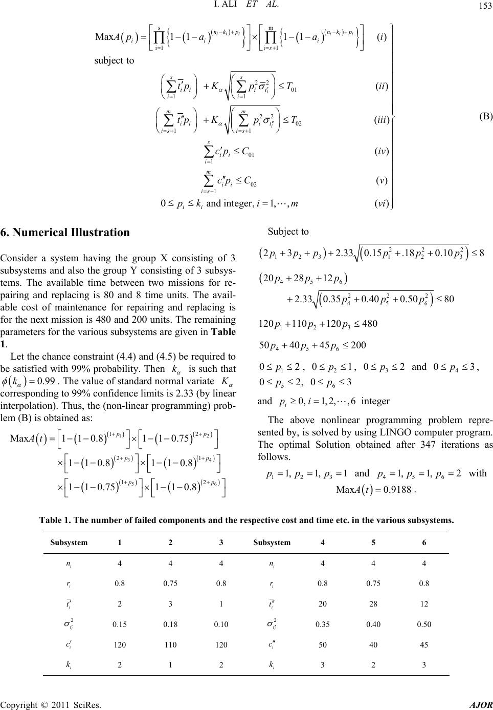
So in subsystem 1, 2 and 3 we replace 1, 1 and 1
components respectively while in the subsystems 4, 5
and 6 we repair and then replace 1, 1 and 2 components
respectively.
7. Conclusions
This paper has provided a profound study of the selective
maintenance problem for an optimum allocation of re-
pairable and replaceable components in system availabil-
ity as a problem of non-linear stochastic programming in
which we maximize the system availability under the
upper bounds on maintenance (i.e., repair and replace)
time and cost. The maintenance time considered as a
random variable and has normal distribution. An equiva-
lent deterministic form of the stochastic non-linear pro-
gramming problem (SNLPP) is established by using the
chance constrained programming problem. Many authors
have solved the allocation of repairable component
problem. But to solve the above problem with probabil-
istic maintenance time will be much more helpful to
demonstrate the practically complicated situations related
to system maintenance problem.
8. References
[1] W. F. Rice, C. R. Cassady and J. A. Nachlas, “Optimal
Maintenance Plans under Limited Maintenance Time,”
Proceedings of the 7th Industrial Engineering Research
Conference, Banff, 9-10 May 1998.
[2] C. R. Cassady, E. A. Pohl and W. P. Murdock, “Selective
Maintenance Modeling for Industrial Systems,” Journal
of Quality in Maintenance Engineering, 2001, Vol. 7, No.
2, pp. 104-117. doi:10.1108/13552510110397412
[3] C. R. Cassady, W. P. Murdock and E. A. Pohl, “Selective
Maintenance for Support Equipment Involving Multiple
Maintenance Actions,” European Journal of Operational
Research, Vol. 129, No. 2, 2001, pp. 252-258.
doi:10.1016/S0377-2217(00)00222-8
[4] C. R. Cassady, E. A. Pohl and J. Song, “Managing Avail-
ability Improvement Efforts with Importance Measures
and Optimization,” IMA Journal of Management Mathe-
matics, Vol. 15, No. 2, 2004, pp. 161-174.
doi:10.1093/imaman/15.2.161
[5] A. Prekopa, “Stochastic Programming,” Series: Mathe-
matics and Its Applications, Kluwer Academic Publishers,
Dordrecht, 1995.
[6] A. Charnes and W. W. Cooper, “Deterministic Equiva-
lents for Optimizing and Satisfying under Chance Con-
straints,” Operations Research, Vol. 11, No. 1, 1963, pp.
18-39. doi:10.1287/opre.11.1.18
[7] S. S. Rao, “Optimization Theory and Applications,” Wiley
Eastern Limited, New Delhi, 1979.
[8] A. Prekopa, “The Use of Stochastic Programming for the
Solution of the Some Problems in Statistics and Probabil-
ity,” Technical Summary Report #1834, University of
Wisconsin-Madison, Mathematical Research Center, Ma-
dison, 1978.
[9] S. Uryasev and P. M. Pardalos, “Stochastic Optimization,”
Kluwer Academic Publishers, Dordrecht, 2001.
[10] F. Louveaux and J. R. Birge, “Stochastic Integer Pro-
gramming: Continuity Stability Rates of Convergence,”
In: C. A. Floudas and P. M. Pardalos, Eds., Encyclopedia
of Optimization, Vol. 5, Kluwer Academic Publishers,
Dordrecht, 2001, pp. 304-310.
[11] G. B. Dantzig, “Linear Programming under Uncertainty,”
Management Science, Vol. 1, No. 3-4, 1955, pp. 197-206.
doi:10.1287/mnsc.1.3-4.197
[12] A. Charnes and W. W. Cooper, “Chance Constrained
Programming,” Management Science, Vol. 6, No. 1, 1959,
pp. 73-79. doi:10.1287/mnsc.6.1.73
[13] V. A. Bereznev, “A Stochastic Programming Problem
with Probabilistic Constraints,” Engineering Cybernetics,
Vol. 9, No. 4, 1971, pp. 613-619.