 American Journal of Oper ations Research, 2011, 1, 73-83 doi:10.4236/ajor.2011.13011 Published Online September 2011 (http://www.SciRP.org/journal/ajor) Copyright © 2011 SciRes. AJOR Higher Order Iteration Schemes for Unconstrained Optimization Yangyang Shi1, Pingqi Pan2 1Faculty of Electrical Engineering, Mathematics and Computer Science, Delft University of Technology, Delft, The Netherlands 2Department of Mat hem at i cs, S o ut heast University, Nanjing, China E-mail: shiyang1983@gmail.com, panpq@seu.edu.cn Received August 3, 2011; revised August 20, 2011; accepted September 19, 2011 Abstract Using a predictor-corrector tactic, this paper derives new iteration schemes for unconstrained optimization. It yields a point (predictor) by some line search from the current point; then with the two points it constructs a quadratic interpolation curve to approximate some ODE trajectory; it finally determines a new point (correc- tor) by searching along the quadratic curve. In particular, this paper gives a global convergence analysis for schemes associated with the quasi-Newton updates. In our computational experiments, the new schemes us- ing DFP and BFGS updates outperformed their conventional counterparts on a set of standard test problems. Keywords: Unconstrained Optimization, Iteration Scheme, ODE Method, Quasi-Newton Update, Convergence Analysis 1. Introduction Consider the unconstrained optimization problem min , n xx R (1) where :n RR is twice continuously differentiable. Let k be the k-th iteration point. We will denote values of () x and its gradient at k by k and k , respectively. Optimization problems are usually solved by iteration methods. The line search widely used in unconstrained optimization is a kind of iteration scheme for updating iterates. Such a scheme, by which one obtains the next iterate 1k from a current iterate k , is of the follow- ing form: 1= kk , k xp (2) where k and p are termed search direction and step- size, respectively. k is usually determined as a descent direction with respect to the objective p() x, and by exact or inexact line searches, so that the objective value decreases after the iteration. For instance, the famous Newton method uses the scheme with search direction 1 2 =, kk pf k f where 2k is the Hessian matrix of () x at k , and stepsize =1 . The quasi-Newton methods are reliable and efficient in solving the unconstrained optimization problems. Saving explicit calculations of the second order deriva- tives and solution of a system of linear equations, quasi-Newton methods achieved a great degree of popu- larity since the first paper of Davidon [1,2]. He used =, kk pHf k where k is some approximation to the inverse Hes- sian matrix 1 2k . The next approximate inverse Hessian matrix 1k , is obtained by updating k by rank-one or rank-two matrix. To this end, all quasi-Newton updates require 1k for satisfying the so-called quasi-Newton equa- tion: 1=, kk k ys (3) where 1k = kk yf f and 1k = kk xx . Various quasi-Newton updates were proposed in the past. The important modification of Davidon’s work by Fletcher and Powell [3] (the DFP algorithm) was the first and successful one. It was then surpassed by the BFGS update (as accepted as the best quasi-Newton method) [4-8] proposed independently by Broyden, Fletcher, Goldfarb and Shanno. These updates theoretically guar- antee all k to be positive definite; therefore, the asso-  74 Y. Y. SHI ET AL. ciated k is a descent direction, and the objective de- creases if p is determined by some line search. There are other iteration schemes that appear differ- ently from the conventional ones. The so-called ODE methods use the following initial value problem: 0 d= d d0= xpx t (4) Assume that satisfies certain conditions, and hence the preceding defines a trajectory. ()px Arrow, Huwicz and Uzawa [9] used ()= ()pxfx and . The associated trajec- tories might be called steepest descent curve and Newton curve respectively [10]. In this way, in fact, one could obtain many curves corresponding to existing uncon- strained optimization methods. 1 2() ()fx fx ()px= Pan [11-13] generalized the steepest descent curve and Newton curve by setting ()=()()px xAx , where () is called ratio factor and () x direction matrix. He suggested some concrete ratio factors and direction matrices, and showed that under certain conditions, the objective value decreases strictly along the associated trajectory, the limit point of which is just an optimum. ODE methods treat the optimization problem in the view of trajectory. They use numerical methods to ap- proximately calculate associated trajectory, and finally approach the limit point of the trajectory. When Euler's approach is applied in the ODE method, standard itera- tion schemes are obtained. In fact the standard iteration schemes are originally derived in the direction of de- creasing the objective function value instead of trajectory. Euler's approach is only of the first order precision. So it is possible to apply higher order approach to mimic the trajectory to get higher order iteration scheme than the standard one. In this paper, we derive new iteration schemes along this line. In view of the importance of DFP and BFGS methods, we will focus on iteration schemes with respect to these methods. The paper is organized as follows. Section 2 derives new iteration schemes. Section 3 offers the convergence analysis. Section 4 reports encouraging computational results with a set of problems. 2. Higher Order Iteration Scheme Assume that k is the current iterate. The next iterate 1k will be determined by approximately following the trajectory, defined by (4). Let 1k be a predictor. In- troduce notation 11 ,. kkk kk ppx ppx We construct a quadratic interpolation curve, locally approximating the trajectory as follows: 2 = kk, k tatbtc (5) where satisfy the following conditions: ,, kkk abc 2= kkkk kk atbtcx , , (6a) 2= kk kk at bp (6b) 211 = kk kkkk atbtcx 1 , 1 . (6c) 1 2= kkk k atb p (6d) Set 1, so =0 k t 1 (0) =k x 1 = kk bp . From (6a)-(6d), it is eas- ily to draw that = k c, and 1k x 11 = 2 kk kkk pp txx , (7a) 1 = 2 kk kk pp at . (7b) Pre-multiplying the both sides of (7a) by , we obtain an approximate 1k, furthermore, have an approximate solution of (6a)-(6d). 1 T kk xx t 11 2 1 =, 4 T kk kkkk k kk pp xxpp axx 1 1 , (8) 1 =, = kkkk bpcx (9) where 1kk xx denotes 2-norm of the vector 1kk xx . The unconstrained optimization problem (1) can get a approximate solution by solving the following one-di- mension minimization problem: 2 min=, 0. kkk tfatbtct (10) To solve such problem, we apply the inexact line search rule, furthermore, we modify the sufficient decent condition , T kkk kk xtp fxtpf (11) in this way: 2, T kkkkkk atbtcf ctbfc (12) where (0,1) . 2.1. Modified Inexact Line Search Algorithm The conventional backtracking inexact line search [14] oper ates in th is way. A t the beginning we set . The algorithm will stop if t satisfies the sufficient decent condition. Otherwise, the algorithm will continue with ˆ =tt tt . A modified backtracking inexact line search algorithm Copyright © 2011 SciRes. AJOR  Y. Y. SHI ET AL. 75 was obtained by applying the expression (12) as the suf- ficient decent condition in backtracking line search algo- rithm. Subalgorithm 2.1 modified backtracking inexact line search Step 0. Given , ˆ t , (0,1) , ; set . ˆ =tt T Step 1. Set if =0 k a> kk kk af cbf T , where con- stant 1 ˆ ct . Step 2. If 2, T kkkkkk atbtcf ctbfc (13) go to step 4; ot herwise, go to ste p 3. Step 3. tt an d go to step 2. Step 4. Terminate with . = k tt 2.2. Higher Order Iteration Schemes The higher order iter ation schemes, firstly obtain the pr e- dictor 1k from the current point k by inexact line search rule following the direction k. Then construct the quadratic interpolation curve by the relevant infor- mation of k p and 1k , and calculate 1k satisfying modified inexact line search rule (12). The overall steps of the higher order iteration schemes are organized as follows. Algorithm 2.1 Higher order iteration schemes Step 0. Given initial point x0, , (0,1) d an , set :=k0; Step 1. If < k f , stop. Step 2. compute the predictor Call backtracking inexact line search algorithm to ob- tain t. k Compute k1= kkk xtp . Step 3. If 1<fx k Step 4. Compute a new iteration point. , stop. Compute ,,abc by (8) and (9). kkk Call subalgorithm 2.1 to get . 1k t Compute 2 111 = k kkkkk at bt := 1kkc . Step 5. Set and go to step 1. 2.3. An Extension of the Higher Order Iteration Scheme The higher order iteration schemes vary with different . In this paper we extend the higher order iteration schemes to BFGS method, and set k . We get the predictor 1k ()px = kk pHf from k , satisfying the back- tracking inexact line search rule, in the direction . From k k p and 1k , we compute 111kk . Then by searching along the curve, we obtain the new point = k pH f 1k . The overall steps of the variant of the itera- tion schemes are organized as follows. Algorithm 2.2 higher order iteration schemes using BFGS upda te Step 0. Given initial point x0; set , := 0k , (0,1) , N, 0= I, and ; Step 1. Compute the predictor. Call backtracking inexact line search algorithm to ob- tain t. k C ompute k1= kkkk xtHf and . 11 = kk ffx Step 2. If 1<fx k , stop. Step 3. Comp ut e 1k . If T kk ys then 1= k I ; otherwise 1=1 TTT kkk kkkkkkkk kk TT T kk kkkk yHy sssyHHys HH sy sysy , T (14) where 1k = kk ff , = kkkk tH f . Step 4. Compute the new iteration point. C ompute ,,abc by (8) and (9). kkk Call subalgorithm 2.1 to get . 1k t C ompute 2 111 = k kkkkk at bt c . Step 5. If 1<fk Step 6. Update , stop. k . If 1( )kmodN= 0 or T kk ys then 1= k I ; oth- erwise 1=1 TTT kkkkkkkkkkk kk TT T kk kkkk yHy sssyHHys HH sy sysy , T f (15) where 1 = kk yf k , 1 = kk k xx . If 11 1 111 < T kk k kkk fH f fHf or 11 1 < T kk k fH f , then set 1= k I . Step 7. Set := 1kk and go to step 1. Note: 1) In this paper, denotes identity matrix. 2) In step 3, we adopt a strategy to make sure that the curvature condition > T kk ys is hold. So 1k is posi- tive and 1k is a decent direction. 3) In step 4, we call the subalgorithm (2.1), in which we set the parameter 1 =c . 4) In step 6, we adopt a restart technique that if 1k is the integral multiple of the N or T kk ys , we restart with 1= k I . Clearly, the BFGS method is a kind of conjugate direction method, so the restart technique can reduce the accumulation of the roundoff errors. 5) We only report the variant using BFGS update. we also derive a variant of the higher order iteration schemes by using the DFP updating formula instead of the BFGS Copyright © 2011 SciRes. AJOR  76 Y. Y. SHI ET AL. updating formula in step 3 and step 6. 3. The Global Convergence of the Higher Order Iteration Schemes Definition 3.1 [11] Curve () t where (0, )t , if for any >0 , (0, )t , () t is conta ined in the domain of and is strictly monotone decreasing in ()fx (0, )(())fxt , then () t is a decent trajectory of at ()fx0 (0) = x. And if lim() t t is exist and equal the minimization point of , then the curve ()fx () t is normal decent trajectory of at ()fx 0 . Pan proved the global convergence of the ODE meth- ods with ratio factor and direction matrix [11]. In this paper we only consider the situation that ratio factor is 1 and direction matrix is identity matrix. So we draw the theorem as follows, Theorem 3.1 [11] Given 0n x , assume the level set 0 =: , n xfxfx is bounded close set, and is twice continuously differentiable in the set and 0, then the right segment trajectory of the the ordinary equations (4) is the decent curve of at 0 ()fx ) ()0 fx ( fx and the limit point of the trajectory is the stationery point of () x. If is convex, then the right segment trajectory is normal decent curve of at ()fx ()fx 0 . We use the quadratic interpolation curve (5) to ap- proximate the trajectory. However, when , the iteration scheme may not be decent in the local re- gion of the predictor 1k >0 T kk af . So we apply the strategy of step 1 in subalgorithm (2.1) to keep the iteration decent. Theorem 3.2 Given constant and ˆ t1 ˆ ct . In subal- gorithm (2.1), if is decent direction satisfying k b 0, T kk bf then for any 1 0<tc , the condition 20, T kk k at btf is hold. Proof. If , clearly, the conclusion holds. 0 T kk af >0 T af Otherwise , from algorithm (2.1) step 1, if kk >, TT kk kk af cbf then set , so the conclusion holds. If =0 k a , TT kk kk af cbf then 210. T T kkkkkk atbtfta bf c □ Theorem 3.3 Consider the algorithm (2.1), where k and k are decent direction, and k satisfying the con- dition p p p 1 T kk kk pf c pf (16) and 2k pcf k (17) where 1 and 2 are constants. Suppose that >0c>0c () x is bounded below and continuously differentiable in the level set 0 =: , n xxfx fx, (18) where 0 is the starting point. And the gradient is Lipschitz continuous on ; namely, there exists L such that . xfyLxy (19) Then for some , k=0 k f is hold, otherwise, lim=0. k kf (20) Proof. Consider the situation that for all k, 0 k f . Then from the algorithm (2.1), we have that 1, T kkkkk ftpf (21) and 11111 , T kk kkkk 1 ftpff (22) By (21) and (22), we have 1, T kk kkk ftp f (23) and 11 0. kk ff (24) With (23) and (24) , we obtain 1. T kk kkk ftp f (25) By summing this expression over all indices less than or equal to k, we obtain 01 =0 . kT kkk jk ftp f (26) Since f is bounded below, we have that 01k f is less than some positive constant, for all k. Hence, by taking limits in (26), we obtain Copyright © 2011 SciRes. AJOR  Y. Y. SHI ET AL. 77 . =0 < T kkk j tpf (27) In standard inexact line search algorithem, we know that if the initiate trial does not satisfy the condition ˆ t (11), then k t violate the condition. So >. T kk kkk k tt k xpf pf (28) By the Lipschitz condition (37), we have 1 0 2 0 2 2 2 = =d d 1 =2 21 , for all 0< kk kkkk tT k T kk kkkkk tk T kk kk T kk kk k T kk T kk kk k fffxtpf tpff xspfps tp fsLps tpfLt p pf tp ftLp (29) It follows from (28) and (29) that 2 21 > T kk k k pf t Lp . (30) If initiate trial satisfy the condition (11), then . Furthermore, from (16) and (17), we have ˆ tˆ = tt 2 21 ˆ min,> 0. T kk k k pf t Lp t (31) It follows fro m (27) that 2 2 =0 21| | ˆ min, < T kk T kk jk pf tp f Lp (32) It follows from (16) and (17) 22 2 112 =0 21 ˆ min, < kk j cptcc f L (33) By (33), we obtain that 2 =0 < k j f . (34) This implies that =0. lim k kf (35) The theorem (3.3) analyzes the global convergence of the iteration scheme based on ODE, similarly, we obtain the global convergence of the variant iteration scheme using BFGS update formula. Theorem 3.4 Consider the algorithm (2.2), suppose that f is bounded below in and continuously differ- entiable in the level set n 0 =xf xf x, (36) where 0 is the starting point. And the gradient is Lipschitz continuous on ; namely, there exists L such that . xfyLxy (37) Then for some , k=0 k f is hold, otherwise, =0. lim k kf (38) Proof. Consider the situation that for all k, 0 k f . Then from the algorithm (2.2), we have that 11 11 T kkkkk1 ftHf f k (39) and 1. T kk kk ftHff (40) The step 3 implies that 11 1 >0 T kk k Hf f (41) By combining the condition (39), (40) and (41), we have 1. T kkkk k ftHf f (42) From the step 8 in the algorithm (2.2), we have that 11 1 111 , T kkk kkk fH f fHf (43) and 11 1 . T kk k fH f (44) From the theorem (3.3), we conclude that =0. lim k kf (45) is hold. □ 4. Computational Results In this section, we report computational results showing that the variant iteration schemes using BFGS and DFP update formula outperformed the BFGS method and DFP method on two sets of test functions. The first set of 20 functions were from [15], and the second from [16], which can be obtained from http://www.ici.ro/camo/neculai/ ansoft.htm. Copyright © 2011 SciRes. AJOR 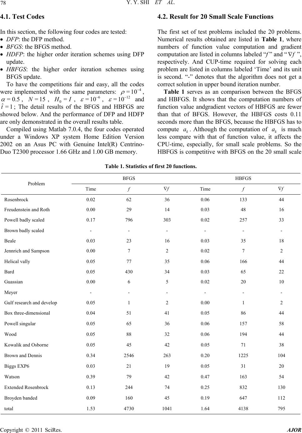 Y. Y. SHI ET AL. Copyright © 2011 SciRes. AJOR 78 4.1. Test Codes 4.2. Result for 20 Small Scale Functions In this section, the following four codes are tested: The first set of test problems included the 20 problems. Numerical results obtained are listed in Table 1, where numbers of function value computation and gradient computation are listed in columns labeled “f ” and “ ”, respectively. And CUP-time required for solving each problem are listed in columns labeled ‘Time’ and its unit is second. “-” denotes that the algorithm does not get a correct solution in upper bound iteration number. DFP: the DFP method. BFGS: the BFGS method. HDFP: the higher order iteration schemes using DFP update. HBFGS: the higher order iteration schemes using BFGS update. To have the competitions fair and easy, all the codes were implemented with the same parameters: 4 =10 , =0.5 , , 0 =15N= I, , 6 =10 12 =10 and ; The detail results of the BFGS and HBFGS are showed below. And the performance of DFP and HDFP are only demonstrated in the overall result s table. ˆ=1 t Compiled using Matlab 7.0.4, the four codes operated under a Windows XP system Home Edition Version 2002 on an Asus PC with Genuine Intel(R) Centrino- Duo T2300 processor 1.66 GHz and 1.00 GB memory. Table 1 serves as an comparison between the BFGS and HBFGS. It shows that the computation numbers of function value andgradient vectors of HBFGS are fewer than that of BFGS. However, the HBFGS costs 0.11 seconds more than the BFGS, because the HBFGS has to compute k. Although the computation of k is much less compare with that of function value, it affects the CPU-time, especially, for small scale problems. So the HBFGS is competitive with BFGS on the 20 small scale a a Table 1. Statistics of first 20 functions. BFGS HBFGS Problem Time f Time f Rosenbrock 0.02 62 36 0.06 133 44 Freudenstein and Roth 0.00 29 14 0.03 48 16 Powell badly scaled 0.17 796 303 0.02 257 33 Brown badly scaled - - - - - - Beale 0.03 23 16 0.03 35 18 Jennrich and Sampson 0.00 7 2 0.02 7 2 Helical vally 0.05 77 35 0.06 166 44 Bard 0.05 430 34 0.03 65 22 Guassian 0.00 6 5 0.02 20 10 Meyer - - - - - - Gulf research and develop 0.05 1 2 0.00 1 2 Box three-dimensional 0.04 51 41 0.05 86 44 Powell singular 0.05 65 36 0.06 157 58 Wood 0.05 88 32 0.06 194 44 Kowalik and Osborne 0.05 45 42 0.05 71 38 Brown and Dennis 0.34 2546 263 0.20 1225 104 Biggs EXP6 0.03 21 19 0.05 31 20 Watson 0.39 79 42 0.47 163 54 Extended Rosenbrock 0.13 244 74 0.25 832 130 Broyden banded 0.09 160 45 0.19 647 112 total 1.53 4730 1041 1.64 4138 795 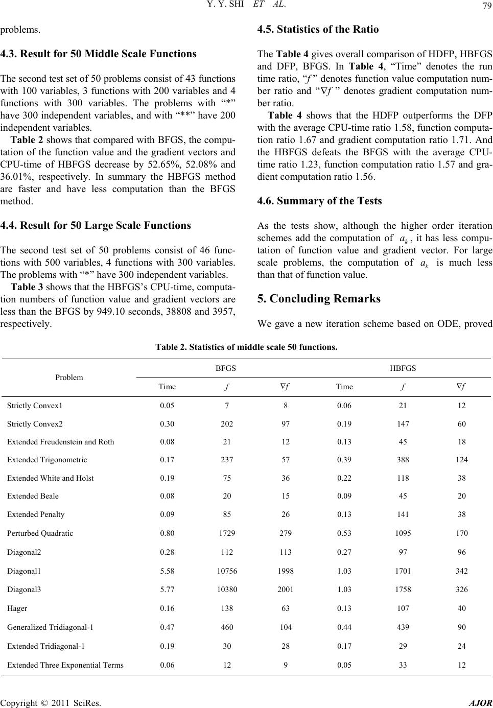 Y. Y. SHI ET AL. Copyright © 2011 SciRes. AJOR 79 problems. 4.3. Result for 50 Middle Scale Functions The second test set of 5 0 problems consis t of 43 functions with 100 variables, 3 functions with 200 variables and 4 functions with 300 variables. The problems with “*” have 300 ind ependen t variables, and with “**” have 200 independe nt variables. Table 2 shows that compared with BFGS, the compu- tation of the function value and the gradient vectors and CPU-time of HBFGS decrease by 52.65%, 52.08% and 36.01%, respectively. In summary the HBFGS method are faster and have less computation than the BFGS method. 4.4. Result for 50 Large Scale Functions The second test set of 50 problems consist of 46 func- tions with 500 variables, 4 functions with 300 variables. The problems with “*” have 300 inde pendent variabl e s. Table 3 shows that the HBFGS’s CPU-time, computa- tion numbers of function value and gradient vectors are less than the BFGS by 949.10 seconds, 38808 and 3957, respectively. 4.5. Statistics of the Ratio The Table 4 gives overall comparison of HDFP, HBFGS and DFP, BFGS. In Table 4, “Time” denotes the run time ratio, “f ” denotes function value computation num- ber ratio and “ ” denotes gradient computation num- ber ratio. Table 4 shows that the HDFP outperforms the DFP with the average CPU-time ratio 1.58, function co mputa- tion ratio 1.67 and gradient computation ratio 1.71. And the HBFGS defeats the BFGS with the average CPU- time ratio 1.23, function computation ratio 1.57 and gra- dient com put at i on rat i o 1.56. 4.6. Summary of the Tests As the tests show, although the higher order iteration schemes add the computation of k, it has less compu- tation of function value and gradient vector. For large scale problems, the computation of is much less than that of function value. a k a 5. Concluding Remarks We gave a new iteration scheme based on ODE, proved Table 2. Statistics of middle scale 50 functions. BFGS HBFGS Problem Time f Time f Strictly Convex1 0.05 7 8 0.06 21 12 Strictly Convex2 0.30 202 97 0 .19 147 60 Extended Freudenstein an d R o t h 0 .08 21 12 0.13 45 18 Extended Trigonometric 0.17 237 57 0.39 388 124 Extended White and Holst 0.19 75 36 0.22 118 38 Extended Beale 0.08 20 15 0.09 45 20 Extended Penalty 0.09 85 26 0.13 141 3 8 Perturbed Quadratic 0.80 1729 279 0.53 1095 170 Diagonal2 0.28 112 113 0.27 97 96 Diagonal1 5.58 10756 1998 1.03 1701 342 Diagonal3 5.77 10380 2001 1.03 1758 326 Hager 0.16 138 63 0.13 107 40 Generalized Tridiagonal-1 0.47 460 104 0.44 439 90 Extended Tridiagonal-1 0.19 30 28 0.17 29 24 Extended Three Exponential Terms 0.06 12 9 0.05 3 3 12  80 Y. Y. SHI ET AL. Generalized Tridiagonal-2 0.67 1261 189 0.77 1340 192 Diagonal4 0.03 9 4 0.03 28 6 Diagonal5 0.03 5 6 0.03 12 8 Extended Himmelblau 0.06 19 10 0.06 56 18 Generalized PSC1 0.73 369 313 0.28 137 104 Extended PSC1 0.06 22 15 0.09 41 22 Extended Powell** 1.45 148 78 0.98 111 50 Extended Block Diagonal BD1 0.05 14 13 0.06 30 16 Extended Maratos 0.19 146 67 0.25 264 90 Extended Cliff 0.17 71 44 0.09 65 22 Quadratic Diagonal Perturbed 0.11 57 40 0.13 65 42 Extended Wood** 0.34 81 25 0.64 134 44 Scaled Quadratic SQ1** 6.61 3163 460 5.70 32 05 360 Quadratic Function QF1 0.52 1015 193 0.42 784 140 Extended Quadratic Penalty QP1 0.06 41 21 0.06 45 16 Extended Quadratic Penalty QP2 0.08 49 26 0.11 82 34 A Quadratic Function QF2 0.92 2352 324 0.58 137 7 186 Extended EP1 0.03 12 5 0.05 31 8 Extended Tridiagonal-2 0.11 75 40 0.11 83 38 BDQRTIC 1.70 5044 560 0.69 1619 206 TRIDIA 1.75 5288 570 0.88 2336 258 ARWHEAD 1.69 749 121 1.81 748 114 NONDIA (Shanno-78) 0.06 88 19 0.19 378 58 NONDQUAR 5.25 2170 1999 2.86 1207 1040 DQDRTIC 0.05 49 13 0.14 234 42 Extended Rosenbrock 0.13 74 38 0.16 153 52 EG2 0.05 21 12 0.08 57 24 DIXMAANA* 0.48 14 11 0.75 27 16 DIXMAANB* 0.69 19 16 0.94 31 20 Almost Perturbed Quadratic 0.80 1744 280 0.47 963 148 Tridiagonal Perturbed Quadratic 1.25 1686 267 0.83 1088 168 DIXMAANC* 0.67 21 16 0.98 40 20 DIXMAANE* 8.31 176 174 4.93 109 102 Partial Perturbed Quadratic 0.97 1618 260 0.64 1019 158 Broyden Tridiagonal 0.64 1030 174 0.66 1015 160 total 50.97 52964 11251 32.31 25078 5392 Copyright © 2011 SciRes. AJOR 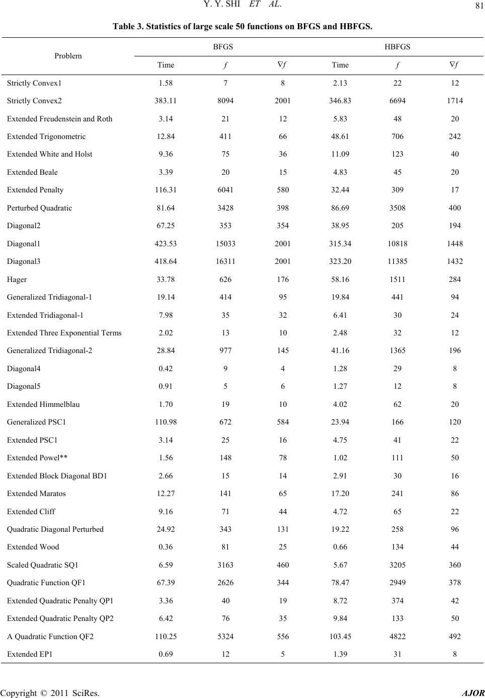 Y. Y. SHI ET AL. 81 Table 3. Statistics of large scale 50 functions on BFGS and HBFGS. BFGS HBFGS Problem Time f Time f Strictly Convex1 1.58 7 8 2.13 22 12 Strictly Convex2 383.11 8094 2001 346.83 6694 1714 Extended Freudenstein an d R o t h 3.14 21 12 5.83 48 20 Extended Trigonometric 12.84 411 66 48.61 706 242 Extended White and Holst 9.36 75 36 11.09 123 40 Extended Beale 3.39 20 15 4.83 45 20 Extended Penalty 116.31 6041 580 32.44 309 17 Perturbed Quadratic 81.64 3428 398 86.69 3508 400 Diagonal2 67.25 353 354 38.95 205 194 Diagonal1 423.53 15033 2001 315.34 10818 1448 Diagonal3 418.64 16311 2001 323.20 11385 1432 Hager 33.78 626 176 58.16 1511 284 Generalized Tridiagonal-1 19.14 414 95 19.84 441 94 Extended Tridiagonal-1 7.98 35 32 6.41 30 24 Extended Three Exponential Terms 2.02 13 10 2.48 32 12 Generalized Tridiagonal-2 28.84 977 145 41.16 1365 196 Diagonal4 0.42 9 4 1.28 29 8 Diagonal5 0.91 5 6 1.27 12 8 Extended Himmelblau 1.70 19 10 4.02 62 20 Generalized PSC1 110.98 672 584 23.94 166 120 Extended PSC1 3.14 25 16 4.75 41 22 Extended Powel** 1.56 148 78 1.02 111 50 Extended Block Diagonal BD1 2.66 15 14 2.91 30 16 Extended Maratos 12.27 141 65 17.20 241 86 Extended Cliff 9.16 71 44 4.72 65 22 Quadratic Diagonal Per turbed 24.92 343 131 19.22 258 96 Extended Wood 0.36 81 25 0.66 134 44 Scaled Quadratic SQ1 6.59 3163 460 5.67 3205 360 Quadratic Function QF1 67.39 2626 344 78.47 2949 378 Extended Quadratic Penalty QP1 3.36 40 19 8.72 374 42 Extended Quadratic Penalty QP2 6.42 76 35 9.84 133 50 A Quadratic Function QF2 110.25 5324 556 103.45 4822 492 Extended EP1 0.69 12 5 1.39 31 8 Copyright © 2011 SciRes. AJOR 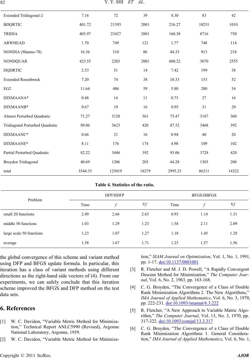 Y. Y. SHI ET AL. Copyright © 2011 SciRes. AJOR 82 Extended Tridiagonal-2 7.16 72 39 8.30 83 42 BDQRTIC 401.72 21393 2001 216.27 10251 1010 TRIDIA 403.97 23427 2001 160.38 8716 750 ARWHEAD 1.70 749 121 1.77 748 114 NONDIA (Shanno-78) 16.36 310 86 44.33 913 218 NONDQUAR 423.55 2203 2001 600.22 3070 2555 DQDRTIC 2.53 51 14 7.42 199 38 Extended Rosenbrock 7.20 74 38 10.33 153 52 EG2 11.64 486 59 5.80 280 34 DIXMAANA* 0.48 14 11 0.73 27 16 DIXMAANB* 0.67 19 16 0.95 31 20 Almost Perturbed Quadratic 71.27 3120 361 75.47 3187 360 Tridiagonal Pert u r be d Q u ad ratic 89.06 3623 420 87.52 3468 392 DIXMAANC* 0.66 21 16 0.94 40 20 DIXMAANE* 8.11 176 174 4.98 109 102 Partial Perturbed Quadratic 82.22 3446 392 93.06 3728 420 Broyden Tridiagonal 40.69 1206 203 44.28 1303 208 total 3544.33 125019 18279 2995.23 86211 14322 Table 4. Statistics of the ratio. DFP/HDFP BFGS/HBFGS Problem Time f Time f small 20 functions 2.49 2.66 2.63 0.93 1.14 1.31 middle 50 functions 1.03 1.29 1.23 1.58 2.11 2.09 large scale 50 functions 1.23 1.07 1.27 1.18 1.45 1.28 average 1.58 1.67 1.71 1.23 1.57 1.56 the global convergence of this scheme and variant method using DFP and BFGS update formula. In particular, this iteration has a class of variant methods using different directions as the right-hand side vectors of (4). From our experiments, we can safely conclude that this iteration scheme improved the BFGS and DFP method on the test data sets. 6. References [1] W. C. Davidon, “Variable Metric Method for Minimiza- tion,” Technical Report ANLC5990 (Revised), Argonne National Laboratory, Argonne, 1959. [2] W. C. Davidon, “Variable Metric Method for Minimiza- tion,” SIAM Journal on Optimization, Vol. 1, No. 1, 1991, pp. 1-17. doi:10.1137/0801001 [3] R. Fletcher and M. J. D. Powell, “A Rapidly Convergent Descent Method for Minimization,” The Computer Jour- nal, Vol. 6, No. 2, 1963, pp. 163-168. [4] C. G. Broyden, “The Convergence of a Class of Double Rank Minimization Algorithms 2. The New Algorithms,” IMA Journal of Applied Mathematics, Vol. 6, No. 3, 1970, pp. 222-231. doi:10.1093/imamat/6.3.222 [5] R. Fletcher, “A New Approach to Variable Matric Algo- rithm,” The Computer Journal, Vol. 13, No. 3, 1970, pp. 317-322. doi:10.1093/comjnl/13.3.317 [6] C. G. Broyden, “The Convergence of a Class of Double Rank Minimization Algorithms 1. General Considera- tion,” IMA Journal of Applied Mathematics, Vol. 6, No. 1,  Y. Y. SHI ET AL. 83 1970, pp. 76-90. doi:10.1093/imamat/6.1.76 [7] D. Goldfarb, “A Family of Variable Metric Methods De- rived by Variational Means,” Mathematics of Computa- tion, Vol. 24, No. 109, 1970, pp. 23-26. doi:10.1090/S0025-5718-1970-0258249-6 [8] D. F. Shanno, “Conditioning of Quasi-Newton Methods for Function on Minimization,” Mathematics of Compu- tation, Vol. 24, No. 111, 1970, pp. 647-656. doi:10.1090/S0025-5718-1970-0274029-X [9] K. J. Arrow, L. Hurwicz and H. Uzawa, “Studies in Lin- ear and Nonlinear Programming,” Stanford University Press, Palo Alto, 1958. [10] F. H. Branin and S. K. Hoo, “A Method for Finding Mul- tiple Extreme of a Function of n Variables,” In: F. A. Lootsman, Ed., Numerical Method for Nonlinear Opti- mization, Academic Press, Cambridge, 1972. [11] P. Q. Pan, “Differential Equation Methods for Uncon- strained Optimization,” Nanjing University Journal of Computational Mathematics, in Chinese, Vol. 4, 1982, pp. 338-349. [12] P. Q. Pan, “New ODE Methods of Equality Constrained Optimization (1): Equations,” Journal of Computational Mathematics, Vol. 10, No. 1, 1992, pp. 77-92. [13] P. Q. Pan, “New ODE Methods for Equality Constrained Optimization (2): Algorithm,” Journal of Computational Mathematics, Vol. 10, No. 2, 1992, pp. 129-146. [14] J. Nocedal and S. J. Wright, “Numerical Optimization,” Science Press, Beijing, 2006. [15] J. J. More, B. S. Garbow and K. E. Hillstrome, “Testing Unconstrained Optimization Software,” ACM Transac- tions on Mathematical Software, Vol. 7, No. 1, 1981, pp. 17-41. doi:10.1145/355934.355936 [16] N. Andrei, “Unconstrained Optimization Test Function,” Advanced Modeling and Optimization, Vol. 10, No. 1, 2008, pp. 147-161. Copyright © 2011 SciRes. AJOR
|