Paper Menu >>
Journal Menu >>
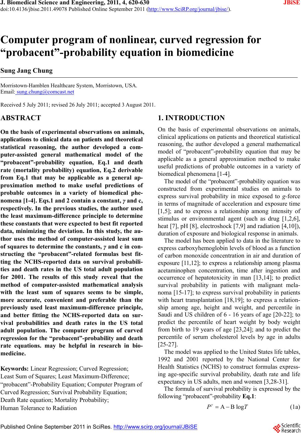 J. Biomedical Science and Engineering, 2011, 4, 620-630 JBiSE doi:10.4136/jbise.2011.49078 Published Online September 2011 (http://www.SciRP.org/journal/jbise/). Published Online September 2011 in SciRes. http://www.scirp.org/journal/JBiSE Computer program of nonlinear, curved regression for “probacent”-probability equation in biomedicine Sung Jang Chung Morristown-Hamblen Healthcare System, Morristown, USA. Email: sung.chung@comcast.net Received 5 July 2011; revised 26 July 2011; accepted 3 August 2011. ABSTRACT On the basis of experimental observations on animals, applications to clinical data on patients and theoretica l statistical reasoning, the author developed a com- puter-assisted general mathematical model of the “probacent”-probability equation, Eq.1 and death rate (mortality probability) equation, Eq.2 derivable from Eq.1 that may be applicable as a general ap- proximation method to make useful predictions of probable outcomes in a variety of biomedical phe- nomena [1 -4]. Eqs.1 and 2 contain a constant, γ and c, respectively. In the previous studies, the author used the least maximum-difference principle to determine these constants that were expected to best fit reported data, minimizing the deviation. In this study, the au- thor uses the method of computer-assisted least sum of squares to determine the constants, γ and c in con- structing the “probacent”-related formulas best fit- ting the NCHS-reported data on survival probabili- ties and death rates in the US total adult population for 2001. The results of this study reveal that the method of computer-assisted mathematical analysis with the least sum of squares seems to be simple, more accurate, convenient and preferable than the previously used least maximum-difference principle, and better fitting the NCHS-reported data on sur- vival probabilities and death rates in the US total adult population. The computer program of curved regression for the “probacent”-probability and death rate equations. may be helpful in research in bio- medicine. Keywords: Linear Regression; Curved Regression; Least Sum of Squares; Least Maximum-Difference; “probacent”-Probability Equation; Computer Program of Curved Regression; Survival Probability Equation; Death Rate equation; Mortality Probability; Human Tolerance to Radiation 1. INTRODUCTION On the basis of experimental observations on animals, clinical applications on patients and theoretical statistical reasoning, the author developed a general mathematical model of “probacent”-probability equation that may be applicable as a general approximation method to make useful predictions of probable outcomes in a variety of biomedical phenomena [1-4]. The model of the “probacent”-probability equation was constructed from experimental studies on animals to express survival probability in mice exposed to g-force in terms of magnitude of acceleration and exposure time [1,5]; and to express a relationship among intensity of stimulus or environmental agent (such as drug [1,2,6], heat [7], pH [8], electroshock [7,9] and radiation [4,10]), duration of exposure and biological response in animals. The model has been applied to data in the literature to express carboxyhemoglobin levels of blood as a function of carbon monoxide concentration in air and duration of exposure [11,12]; to express a relationship among plasma acetaminophen concentration, time after ingestion and occurrence of hepatotoxicity in man [13,14]; to predict survival probability in patients with malignant mela- noma [15-17]; to express survival probability in patients with heart transplantation [18,19]; to express a relation- ship among age, height and weight, and percentile in Saudi and US children of 6 - 16 years of age [20-22]; to predict the percentile of heart weight by body weight from birth to 19 years of age [23,24]; and to predict the percentile of serum cholesterol levels by age in adults [25-27]. The model was applied to the United States life tables, 1992 and 2001 reported by the National Center for Health Statistics (NCHS) to construct formulas express- ing age-specific survival probability, death rate and life expectancy in US adults, men and women [3,28-31]. The formula of survival probability is expressed by the following “probacent”-probability Eq.1: AB logPT (1a) 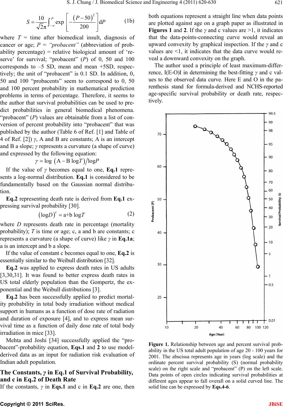 S. J. Chung / J. Biomedical Science and Engineering 4 (2011) 620-630 Copyright © 2011 SciRes. JBiSE 621 2 50 10 exp d 200 2π PP SP (1b) where T = time after biomedical insult, diagnosis of cancer or age; P = “probacent” (abbreviation of prob- ability percentage) = relative biological amount of ‘re- serve’ for survival; “probacent” (P) of 0, 50 and 100 corresponds to –5 SD, mean and mean +5SD, respec- tively; the unit of “probacent” is 0.1 SD. In addition, 0, 50 and 100 “probacents” seem to correspond to 0, 50 and 100 percent probability in mathematical prediction problems in terms of percentage. Therefore, it seems to the author that survival probabilities can be used to pre- dict probabilities in general biomedical phenomena. “probacent” (P) values are obtainable from a list of con- version of percent probability into “probacent” that was published by the author (Table 6 of Ref. [1] and Table of 4 of Ref. [2]) γ, A and B are constants; A is an intercept and B a slope; γ represents a curvature (a shape of curve) and expressed by the following equation: log AB loglogTP If the value of γ becomes equal to one, Eq.1 repre- sents a log-normal distribution. Eq.1 is considered to be fundamentally based on the Gaussian normal distribu- tion. Eq.2 representing death rate is derived from Eq.1 ex- pressing survival probability [30]. c loga+b logDT (2) where D represents death rate in percentage (mortality probability); T is time or age; c, a and b are constants; c represents a curvature (a shape of curve) like γ in Eq.1a; a is an intercept and b a slope. If the value of constant c becomes equal to one, Eq.2 is essentially similar to the Weibull distribution [32]. Eq.2 was applied to express death rates in US adults [3,30,31]. It was found to better express death rates in US total elderly population than the Gompertz, the ex- ponential and the Weibull distributions [3]. Eq.2 has been successfully applied to predict mortal- ity probability in total body irradiation without medical support in humans as a function of dose rate of radiation and duration of exposure [4], and to express mean sur- vival time as a function of daily dose rate of total body irradiation in mice [33]. Mehta and Joshi [34] successfully applied the “pro- bacent”-probability equation, Eqs.1 and 2 to use model- derived data as an input for radiation risk evaluation of Indian adult population. The Constants, γ in Eq.1 of Survival Probability, and c in Eq.2 of Death Rate If the constants, γ in Eqs.1 and c in Eq.2 are one, then both equations represent a straight line when data points are plotted against age on a graph paper as illustrated in Figures 1 and 2. If the γ and c values are >1, it indicates that the data-points-connecting curve would reveal an upward convexity by graphical inspection. If the γ and c values are <1, it indicates that the data curve would re- veal a downward convexity on the graph. The author used a principle of least maximum-differ- rence, I(E-O)I in determining the best-fitting γ and c val- ues to the observed data curve. Here E and O in the pa- renthesis stand for formula-derived and NCHS-reported age-specific survival probability or death rate, respec- tively. Figure 1. Relationship between age and percent survival prob- ability in the US total adult population of age 20 - 100 years for 2001. The abscissa represents age in years (log scale) and the ordinate percent survival probability (S) (normal probability scale) on the right scale and “probacent” (P) on the left scale. Data points of open circles indicating survival probabilities at different ages appear to fall overall on a solid curved line. The solid line can be expressed by Eqs.4-6.  S. J. Chung / J. Biomedical Science and Engineering 4 (2011) 620-630 Copyright © 2011 SciRes. JBiSE 622 Figure 2. Relationship between age and death rate in the US total elderly population of 60 - 100 years for 2001. The ab- scissa represents age in years and the ordinate death rate (D) in percentages (log scale). Data points of closed circles indicate US national life table death rates reported by the National Center for Health Statistics (NCHS) for 2001. The dashed straight line represents death rates predicted by the Gompertz mortality model expressed by equation, D = 10 (-2.2674 + 0.03779T). The solid curved line represents death rates predicted by the “probacent”-probability model of death rate (D) expressed by Eqs.7 and 8. Data points of NCHS appear to fall overall on the solid death-rate line predicted by Eqs.7 and 8. The maximum predictive error of the “probacent” model is ±0.3% and that of the Gompertz model ±3.2%. Source: reference [3]. In analysis of the least maximum-difference, random different values of integer and/or fractional number are substituted as γ and c values in Eq.1 or 2 to calculate survival probabilities, (S) or death rates, (D). The above described method of the least maximum-difference principle was used in the author’s previous publications to minimize the deviation. The least sum of squares of well-known linear regression in statistics [32,35,36] is not employed in the previous author’s studies. However, to my knowledge, there seem to be no computer-pro- gram-assisted, nonlinear, curved regression models of the least sum of squares in the literature that determine the best-fitting constant, γ or c value in the “probacent”- probability or death rate equation, Eq.1 or 2, minimizing the sum of deviation [37-42]. The purpose of this study is to design a computer pro- gram of nonlinear, curved regression of the least sum of squares for construction of best-fitting equations. of “probacent”-probability and death rate developed by the author to the NCHS-reported data [29]. 2. MATERIALS AND METHODS The National Center for Health Statistics reported the United States life tables, 2001 for US total, male and female populations on the basis of 2001 mortality statis- tics, the 2000 decennial census and the data from the Medicare program (E. Arias, United States life tables, 2001, Natl. Vital Stat. Rep. 52 (2004) 1-40 [29]). The author published computer-assisted predictive formulas expressing the NCHS-reported survival prob- abilities, death rates (mortality probabilities) and life expectancies in US adults, men and women, 2001, em- ploying a model of the “probacent”-probability and death- rate equations previously published by the author in the study [3]. The survival probability is percent probability of surviving to the beginning of age T from birth. The death rate is percent probability of dying between age T to T + 1. The data are plotted on a log-log graph paper as illus- trated in Figures 1 and 2. In this study, the data on survival probabilities and death rates shown in the NCHS’ report [29] and [3] as well as Figures 1 and 2 are used to design computer pro- grams of nonlinear, curved regression of the least sum of squares for the “probacent”-probability and death rate equations to minimize the sum of deviations, and to find the best-fitting constant values, γ and c. 2.1. Use of the Least-Maximum-Difference Principle in Analysis In the author’s previous studies, the least maximum- difference principle, least I(E-O)I (the absolute value of the difference) is used to minimize the deviation. 2.1.1. Formulas of Survival Probabilities (S) A mathematical method to determine constants, γ, A and B in Eq.1 is described in Appendix of Ref. [3]. Two sets of data on age (T) and survival probability (S) are used in each age group, 20 - 60, 60 - 85 or 85 - 100 years to determine constants A and B as seen in Eqs.3a, 3b and 3c, respectively. The most appropriate and best- fitting γ values of Eq.1 for the age groups of 20 - 60, 60 - 85, and 85 - 100 years are determined, using the least maximum-difference principle and comparing maximum  S. J. Chung / J. Biomedical Science and Engineering 4 (2011) 620-630 Copyright © 2011 SciRes. JBiSE 623 differences I (E-O) I calculated by substituting a various semi-random and semi-selective values as the γ value in Eqs.3a, 3b and 3c. 4.6767771.0023.67677x61.605 2.63013 71.00261.605log P T (3a) 12.75482 61.60511.7548246.405 6.6107 61.60546.405log P T (3b) 28.3366446.40527.336664 29.538 14.16832 46.40529.538log P T (3c) The following Eqs.4, 5 and 6 are thus constructed to express survival probabilities of the three age groups: The age group of 20 - 60 years: Eqs.4a and 4b. 12.712.7 12.7 12.7 12.7 4.67677 71.0023.67677 61.605 2.63013 71.00261.605log P T (4a) The age group of 60-85 years: Eqs.5a and 5b. 4.84.8 4.8 4.8 4.8 12.75482 61.60511.75482 46.405 6.6107 61.60546.405log P T (5a) The age group of 85-100 years: Eqs.6a and 6b. 2.32.3 2.3 2.3 2.3 28.3366446.40527.3366429.538 14.16832 46.40529.538log P T (6a) 2 50 10 exp d 200 2 PP SP (4b,5b,6b) 2.1.2. Formulas of Death Rates (D) Constants, c, a and b are determined likewise as above described (the author’s note: see Appendix of Reference [33] if needed) and the following equations are con- structed to express death rates of the two age groups: The age group of 60 - 85 years: 0.82 0.82 0.82 0.82 0.82 log=12.75481 0.0065511.75481 0.97102 6.61070.971020.00655 log D T (7) The age group of 85 - 100 years: 1.7 1.7 1.7 1.7 1.7 log=30.136510.9710229.13651 1.42545 15.101181.425450.97102 log D T (8) 2.2. Use of the Least Sum of Squares in Analysis In this study, the least sum of squares is used. 2.2.1. Formulas of Survival Probabilities (S) The method of least sum of squares, least ∑ (E-O)² is used to determine the best-fitting γ and c values of the “probacent”-probability equation to minimize the sum of deviations. Abridged five-year intervals are used for analysis to simplify computer programs. A close look at the data points in Figure 1 in graphic inspection suggests that the line connecting data points at each age group of 20 - 60, 60 - 85 and 85 - 100 years bulges upward, revealing an upward convexity and so that the γ value is >1. If the line shows a straight line, it indicates γ = 1. If the line reveals a downward like the line connecting the data points on death rates of the age group of 60 - 85 years in Figure 2, it would indicate 0 < γ < 1. A three-step approach in analyzing data with help of the computer program is taken to find the best-fitting constant values, γ and c in Eqs.1 and 2. The first step of computer-assisted mathematical analysis: Enter an integer N, starting from 1 and increasing the integer, 2, 3, up to N as the γ value in Eq.3a for the age group of 20 - 60 years in US adults. Sums of squares, Σ (E-O)² are calculated with the computer program shown in Figure 3. The computer-derived line repre- senting Eq.3 with a specific γ value of 1 to N first ap- proaches toward the NCHS-reported-data line from the starting straight line; the sum of squares would be gradually decreasing. When the computer-generated line touches the NCHS-reported-data line, the sum of squares becomes minimum, the least sum, ideally zero. After passing the NCHS-data line, the sum of squares with increasing γ values would suddenly begin to increase and continues to increase further more. These processes are shown in Table 1. The second step of computer-assisted mathematical analysis: If the sum of squares suddenly starts increasing after preceding gradual decrease at integer N + 1 of γ value, then enter N – 0.1 and N + 0.1 as γ value in Eq.3a. Cal- culate the sums of squares. Compare the sums at (N – 0.1) and (N + 0.1) with the sum at N. The third step of computer-assisted mathematical analysis: If the sum at (N – 0.1) is smaller than the sum at N, then enter (N – 1) + 0.1, (N – 1) + 0.2, (N – 1) + 0.9 as γ value in Eq.3a. Compare the sums of squares and choose the number with the least sum of squares that is determined to be the best-fitting γ value for Eq.3a. A very close and best agreement is found between the computer-derived and NCHS-reported survival prob- abilities with the γ value of 12.8. Eqs.9a and 9b, are finally derived to best represent a relationship between  S. J. Chung / J. Biomedical Science and Engineering 4 (2011) 620-630 Copyright © 2011 SciRes. JBiSE 624 Figure 3. The computer program to calculate the sum of squares, Σ (E-O)² as a function of γ value and age (T) in the US total adult population. Results of execution of the program are shown in Ta- bles 1 and 3. This program is for γ value of 12.8 in Eq.4a for the age group of 20 - 60 years.  S. J. Chung / J. Biomedical Science and Engineering 4 (2011) 620-630 Copyright © 2011 SciRes. JBiSE 625 Table 1. Sums of squares of differences, Σ (E-O)² in nonlinear, curved regression of the least sum of squares to determine a best-fitting γ value for the “probacent”-probability equation expressing age-specific survival probabilities (S)a in US total adult popu- lation. Sums of squares of differences are calculated by computer programs. A representative program is illustrated in Figur e 3. Age group 20 - 60 years 60 - 85 years 85 - 100 years Used “probacent” equation Eq.3a Eq.3b Eq.3c Finally chosen γ value (N) 12.8 4.8 2.3 N* ∑ (E-O)² change N ∑ (E-O)² change N ∑ (E-O)² change 1 19.211494 1 141.460900 1 9.451314 2 16.037229 D** 2 76.313722 D** 2 0.478184 D** 3 13.142712 D 3 31.381485 D 3 3.017885 I*** 4 – 11 continue to decrease 4 6.421165 D 12 0.148060 D 5 0.515137 D 1.9 0.855876 # 13 0.086081 D 6 12.296666 I*** 2.1 0.216581 ## 14 0.263210 I*** 4.9 0.283176 # 2.2 0.070861 D 12.9 0.081272 # 5.1 0.924423 ## (2.3) (0.040713) D 13.1 0.093282 ## 2.4 0.125714 I 4.1 4.991807 D 2.5 0.325343 I 12.1 0.130686 D 4.2 3.752168 D 12.2 0.115832 D 4.3 2.701102 D 12.3 0.103485 D 4.4 1.837403 D 12.4 0.093632 D 4.5 1.159808 D 12.5 0.086258 D 4.6 0.666995 D 12.6 0.081349 D 4.7 0.357585 D 12.7 0.078891 D (4.8) (0.230143) D (12.8) (0.078871) D 4.9 0.283176 I 12.9 0.081272 I 5 0.515137 I 13 0.086081 I (S)a:: survival probability is percent probability of surviving to the beginning of age T from birth; *N represents a number, integer or fractional number; ** D indicates that sum, ∑ (E-O)² decreases below the preceding sum; *** I indicates that sum, ∑ (E-O)² increases above the preceding sum; # Compare the sum with the sum at the last number (N) just before its sum starts increasing (see text); ## Compare the sum with the sum at the last number (N) just before its sum starts increasing (see text). age and survival probability in US adults of 20 - 60 years of age. If the sum at (N – 0.1) is larger than the sum at N and the sum at (N + 0.1) is smaller than the sum at N, then enter (N + 0.2), (N + 0.3) as γ value in Eq.3a. Compare the sums of squares and choose the number with the least sum of squares that is the γ value best fit- ting to the data. The equations of survival probabilities, Eqs.10 and 11 for the age groups of 60 - 85 and 85 - 100 years are likewise derived as shown in Table 1. The age group of 20 - 60 years: Eqs.9a and 9b 12.8 12.812.8 12.812.8 =4.67677 71.0023.67677 61.605 2.63013 71.00261.605log P T (9a) The age group of 60-85 years: Eqs.10a and 10b. 4.8 4.84.8 4.8 4.8 =12.75482 61.60511.75482 46.405 6.610761.60546.405 log P T (10a) The age group of 85-100 years: Eqs.11a and 11b. 2.3 2.32.3 2.3 2.3 =28.33664 46.40527.33664 29.538 14.16832 46.40529.538log P T (11a) ² 50 10 exp d 200 2π PP SP (9b, 10b, 11b) Both methods of mathematical analysis, the least- maximum-difference and the least sum of squares give different γ values, 1.7 and 1.8 for the age groups of 20 - 60 years. However, both methods give same γ values, 4.8 and 4.8 for the age group of 60 - 85 years, and 2.3 and 2.3 for the Age Group of 85 - 100 Years. 2.2.2. Formulas of Death Rates (D) The constants c, a and b are likewise derived as ex- plained above and as seen in Ta b l e 2 . Fractional numbers are used to determine these constants. Two following formulas expressing death rates for the age groups of 60 - 85 and 85 - 100 years for the US total elderly population: The age group of 60-85 years: Eq.12. 0.79 0.79 0.79 0.79 0.79 log=12.75481 0.0065511.75481 0.97102 +6.61070.971020.00655 log D T (12) The age group of 85 - 100years, Eq.13. 1.8 1.8 1.8 1.8 1.8 log=30.136510.9710229.13651 1.42545 15.101181.425450.97102 log D T (13)  S. J. Chung / J. Biomedical Science and Engineering 4 (2011) 620-630 Copyright © 2011 SciRes. JBiSE 626 Table 2. Sums of squares of differences, Σ (E-O)² in nonlinear, curved regression of the least sum of squares to determine a best-fitting c value for the death rate equation expressing age-specific death rates (D)a in US total elderly population. Sums of squares of differences are calculated by computer programs. A program es- sentially similar to Figure 3 program is employed. Age group 60 - 85 years 85 - 100 years Used death rate equation Eqs.7, 12 Eq.8, 13 Finally chosen c value (N) 0.79 1.8 N* ∑ (E-O)² change N ∑ (E-O)² change 1.0 0.869088 1.0 0.655987 0.9 0.288493 D** 1.5 0.095908 ** 0.8 0.046072 D 2.0 0.045142 D 0.7 0.209247 I*** 2.5 0.487048 I*** 0.81 0.0 53194 # 1.9 0.015243 # (0.79) (0.043004) ## 2.1 0.094769 ## 0.78 0.044062 I 1.6 0.045436 D 0.77 0.049313 I 1.7 0.015251 D (1.8) (0.005231) D 1.9 0.015243 I 2.0 0.045142 I (D)a: death rate is percent probability of dying between age T to T +1. *N represents a number, integer or fractional number.** D in- dicates that sum, ∑ (E-O)² decreases below the preceding sum. *** I indicates that sum, ∑ (E-O)² increases above the preceding sum. # Compare the sum with the sum at the last number (N) just before its sum starts increasing (see text). ## Compare the sum with the sum at the last number (N) just before its sum starts increasing (see text). Both methods of mathematical analysis, the least maxi- mum-difference and the least sum of squares give dif- ferent c values, 0.82 and 0.79 for the age group of 60 - 85 years, and 1.7 and 1.8 for the age group of 85 - 100 years, respectively. 2.3. Description of the Computer Program The programs were written in UBASIC for IBM PC mi- crocomputer and compatibles for Eqs.3-13. The com- puter program uses a formula of approximation instead of the integral of Eq.1b and Eqs.4b, 5b, 6b, 9b, 10b, 11b) because the computer cannot perform integral [2, 43-45]. Mathematical transformation of integral, Eq.1b to the formula of approximation is described in detail in the author’s book [45]. A representative computer pro- gram is illustrated in Figure 3 to calculate the sum of squares, Σ (E-O)² with the γ value of 12.8 in Eq.9a. 2.4. Statistical Analysis A χ² goodness-of-fit test (logrank test) [35] is used to test the fit of mathematical models to the NCHS-reported data [29]. The differences are considered statistically significant when p < 0.05. 3. RESULTS Tables 3 and 4 show comparison of least maximum- differences, I(E-O)I, least sum of squares, ∑ (E-O)² and χ²-test p value in the two analytical methods of the least maximum-difference and least sum of squares, in age- specific survival probabilities and death rates for US total adult population, calculated by computer programs as shown in a representative program, Figure 3. The γ values in the survival probability equation in both methods are different, 12.7 and 12.8 in Eqs.4a and 9a for the age group of 20 - 60 years but same 4.8 and 4.8 in Eqs.5a and 10a for the age group of 60 - 85 years, 2.3 and 2.3 in Eqs.6a and 11a for the age group of 85-100 years. The c values in the death rate equation in both methods are all different, 0.82 and 0.79 in Eqs.7 and 12, 1.7 and 1.8 in Eqs. 8 and 13 for the age groups of 60 - 85 and 85 - 100 years, respectively. The least maximum-difference and the least sum of squares reveal slightly smaller values in those in the least sum of squares than in the least maximum-difference but same values in Eqs.5 and 10, and Eqs.6 and 11 for the age groups of 60 - 85 and 85 - 100 years. The above re- sults suggest that regression curves of the least sum of squares are closer to the NCHS-data-connecting line than those of the least maximum-difference. The χ²-test p values are all >0.995, suggesting a very close agreement between both values of computer-derived and NCHS-reported survival probabilities and death rates. The above described results seem to indicate that the analytical method of the least sum of squares is simpler, convenient and preferable, and give more accurate in  S. J. Chung / J. Biomedical Science and Engineering 4 (2011) 620-630 Copyright © 2011 SciRes. JBiSE 627 Table 3. Comparison of the least maximum-difference, І(E-O)І, the least sum of squares, Σ (E-O)² and χ²-test p value in the two analytical methods of the least maximum-difference and the least sum of squares in age-specific survival prob- abilities for US total adult population. Age group 20 - 60 years 60 - 85 years 85 - 100 years Used “probacent” equation Eq.4a Eq.9a Eq.5a Eq.10a Eq.6a Eq.11a γ value 12.7 * 12.8** 4.8* 4.8** 2.3* 2.3** Least maximum-Difference, I(E-O)I 0.158 0.148 0.4 0.4 0.2 0.2 Least sum of Squares, ∑ (E-O)2 0.078891 0.0788710.230143 0.2301430.040713 0.040713 χ²-test p value >0.995 >0.995 >0.995 >0.995 >0.995 >0.995 *γ value is obtained by the method of the least maximum-difference, I(E-O)I.. ** γ value is obtained by the method of the least sum of squares of curved regression, Σ (E-O)². ‘E’ indicates computer-derived value of survival probability. ‘O’ indicates NCHS-reported value of survival prob- ability [29] (see text). Table 4. Comparison of the least maximum-difference, І(E-O)І, the least sum of squares, Σ (E-O)² and χ²-test p value in the two analytical methods of the least maximum-difference and the least sum of squares in age-specific death rates for US total elderly population. Age group 6 0 - 85 years 85 - 100 years Used equation Eq.10 Eq.12 Eq.11 Eq.13 γ value 0.82 * 0.79 ** 1.7* 1.8** Least maximum-difference, I(E-O)I 0.359 0.325 0.132 0.073 Least sum of squares, Σ (E-O)² 0.064304 0.043004 0.015280 0.005275 χ²-test p value >0.995 >0.995 >0.995 >0.995 *γ value is obtained by the method of the least maximum-difference principle, I(E-O)I. ** γ value is obtained by the method of the least sum of squares of curved regression, Σ (E-O)² . ‘E’ indicates computer-derived value of survival probability. ‘O’ indicates NCHS-reported value of sur- vival probability [29] (see text). determining values of γ and c constants in the “pro- bacent”-probability and death rate equations. 4. DISCUSSION Comparison of data shown in Tables 3 and 4 suggests a very close agreement between formula-derived and NCHS-reported data on survival probabilities and death rates in US total adult population because χ² - test p val- ues are >0.995 for each equation expressing them. However, The method of the least sum of squares, least ∑ (E-O)² gives more accurate and best fitting val- ues of constants, γ and c in these equations that fit better the NCHS-reported data, closer to the data-points con- necting line. The computer program of curved regression of the least sum of squares for the “probacent”-probability and death rate seems preferable to the method of the least maximum-difference, least I(E-O)I to minimize the deviation. The author feels that in a variety of biological phe- nomena, γ and c values are, if applicable, generally greater than one or less than one but not one, indicating a curved line when plotted on a X-Y graph paper as seen in Fig- ures 1 and 2. The γ and c values are relatively rarely one, indicating a straight line on a graph or otherwise ap- proximately appearing straight. This phenomena seems to be possibly analogous in physics to that light path is actually curved when passing through a gravitational field of space but appears straight [46,47]. If the γ value becomes equal to one, Eq.1 represents a log-normal distribution. If the c value is one, Eq.2 that is derivable from Eq.1 [30] becomes essentially similar to the Weibull distribution [32]. Weibull distribution is a generalized exponential distribution [32]. If the base of a logarithm is one, the lognormal distribution would be- come a normal distribution (log1 1n = n) [45, 48]. If the logarithm of one as its base is taken for X axis of time, the Gompertz distribution might be similar to the Wei- bull distribution. Therefore, it seems to the author that the Gompertz distribution might be a specific form of the “probacent”-probability equation. A normal distribution is likewise a specific form of the “probacent”-probability equation. “probacent” can be a dependent variable versus an independent variable such as time or age as seen in sur- vival probability, death rate and life expectancy in US total adult population (NCHS) [3,29]. “probacent” can be a dependant variable versus two independent vari- ables such as intensity of stimulus or harmful agent and duration of exposure like dose rate of radiation and dura- tion of exposure in total body irradiation [4], and like  S. J. Chung / J. Biomedical Science and Engineering 4 (2011) 620-630 Copyright © 2011 SciRes. JBiSE 628 dose of drug and time after administration [2,14]. In cases of two independent variables, Eq.1 can make a prediction of probability of occurrence of a response in subjects in various biomedical phenomena. The original and ultimate purpose of the author’s studies has been to find a general mathematical model, possibly a mathe- matical law hidden in nature that might calculate the probability of safe survival in humans and other living organisms exposed to any harmful or adverse circum- stances, overcoming the risk [1,45]. The “probacent”-probability does not predict a single definite result or response for an individual observation in biodynamic biological phenomena. Instead, if the same observations are made on a large number of similar population, each of who had the same condition at the start, the model would predict the possible outcomes, the approximate biomedical events in quantities under ob- servations, but it could not predict the occurrence of the specific event in an individual. Thus, the “probacent”- probability would introduce an unpredictability in bio- medicine like an uncertainty principle of Werner Heisen- berg in quantum mechanics [46,47] The computer program represented by Figure 3 can easily calculate survival probabilities that are required to determine the least sum of squares, by using an ap- proximation instead of integral in Eqs.4b, 5b, 6b, 9b, 10b, 11b. This enables users of the “probacent” model in mathematical analysis, to eliminate a need for consulta- tion of table of normal frequency or percentile in books of statistics and mathematics. 5. CONCLUSIONS In this study, a computer program of nonlinear, curved regression of the least sum of squares is designed to de- termine the constant values of γ in Eq.1 and c in Eq.2 that seems better fitting and more accurate than those obtained by the least maximum-difference principle as suggested by the data shown in Ta bles 3 an d 4. The re- gression curve obtained by this method of the least sum of squares is closer to the data-point-connecting line than that obtained by the least maximum-difference principle. The computer program of curved regression for the “probacent”-probability equation may be helpful in re- search in biomedicine. The computer program of curved regression of this study would need further improvement to enable users to readily find the best-fitting constant values in the equations of the “probacent”-probability and death rate. 6. ACKNOWLEDGEMENTS The author thanks Dr. C. W. Sheppard and Bruce Presley for their teachings in computer programming that made the author’s studies possibly published to the academic world. REFERENCES [1] Chung, S.J. (1960) Studies on a mathematical relation- ship between stress and response in biological phenom- ena. Republic of Korea Journal of the National Academy of Sciences, 2, 115-162. [2] Chung, S.J. (1986) Computer-assisted predictive math- ematical relationship among metrazol dose and time and mortality in mice. Computer Methods and Programs in Biomedicine, 22, 275-284. doi:10.1016/0169-2607(86)90004-0 [3] Chung, S.J. (2007) Computer-assisted predictive formu- las expressing survival probability and life expectancy in US adults, men and women, 2001. Computer Methods and Programs in Biomedicine, 86, 197-209. doi:10.1016/j.cmpb.2007.02.009 [4] Chung, S.J. (2011) Predictive formulas expressing dose rate, duration of exposure and mortality probability in total body irradiation in humans. Journal of Biomedical Science and Engineering, 4, 497-505. doi:10.4236/jbise.2011.47063 [5] Chung, S.J. (1959) Studies of positive radial acceleration on mice. Journal of Applied Physiology, 14, 52-54. [6] Boak, H. and Chung, S.J. (1962) Studies on a relation- ship between dose, time and percentage of occurrence of response and a method of evaluation of combined action in drugs. The New Medical Journal, 5, 35-82. [7] Kim, C.C. and Chung, S.J. (1962) Studies on a relation- ship between stress, duration of exposure and percentage of response in goldfish to single, double and triple stresses of acceleration, electroshock, heat, chemical and osmotic stimuli. Republic of Korea Theses of Catholic Medical College, 5, 257-336. [8] Cho, D.W. and Chung, S.J. (1961) Studies of tolerance of Paramecium caudatum to hydrogen and hydroxyl ions. Bulletin of Yamaguchi Medical School, 8, 151-160. [9] Chung, S.J. (1989) Computer-assisted mathematical rela- tionship among electroshock voltage and duration and occurrence of convulsion in mice. Computer Methods and Programs in Biomedicine, 28, 23-30. doi:10.1016/0169-2607(89)90177-6 [10] Cerveny, T.J., MacVittie, T.J. and Young, R.W. (1989) Acute radiation syndrome in humans. Medical Conse- quences of Nuclear Warfare, TMM Publishers, Office of the Surgeon General, Falls Church, Virginia, 15-36. [11] Forbes, W.H., Sergent, F. and Roughton, F.J.W. (1988) The risk of carbon monoxide uptake by normal men. American Journal of Physiology, 143, 594-608. [12] Chung, S.J. (1988) Formula predicting carboxyhemoglo- bin resulting from carbon monoxide exposure. Veterinary and Human Toxicology, 30, 528-532. [13] Prescott, L.F., Roscoe, P., Wright, N. and Brown, S.S. (1991) Plasma paracetamol half-life and hepatic necrosis in patients with paracetamol overdosage. Lancet, I, 519- 522. [14] Chung, S.J. (1989) Computer-assisted predictive math- ematical relationship among plasma acetaminophen con- centration, time after ingestion and occurrence of hepa- totoxicity in man. Computer Methods and Programs in Biomedicine, 28, 37-43.  S. J. Chung / J. Biomedical Science and Engineering 4 (2011) 620-630 Copyright © 2011 SciRes. JBiSE 629 doi:10.1016/0169-2607(89)90179-X [15] Popescu, N.A., Beard, C.M., Winkelman, P.J., O’Brien, P.C. and Kurland, L.T. (1990) Cutaneous malignant melanoma in Rochester, Minnesota: Trends in incidence and survivorship, 1950 through 1985. Clinical Proceed- ings, 65, 1293-1302. [16] Chung, S.J. (1991) Formula predicting survival in pa- tients with invasive cutaneous malignant melanoma. In- ternational Journal of Biomedical Computing, 28, 151- 159. [17] Chung, S.J. (1994) Formula expressing a relationshipp among lesion thickness and time after diagnosis and sur- vival probability in patients with malignant melanoma. International Journal of Biomedical Computing, 37, 171- 180. doi:10.1016/0020-7101(94)90139-2 [18] Kirklin, J.R., Naftel, D.C., Kirklin, J.W., Blackstone, E.H., White-Williams, C. and Bourge, R.C. (1988) Pul- monary vascular resistance and the risk of heart trans- plantation. Journal of Heart Transplantation, 7, 331-336. [19] Chung, S.J. (1993) Formula predicting survival probabil- ity in patients with heart transplantation. International Journal of Biomedical Computing, 32, 211-221. doi:10.1016/0020-7101(93)90015-X [20] Magbool, G., Kaul, K.K., Corea, J.R., Osman, M. and Arfaj, A. (1993) Weight and height of Saudi children six to 16 years from the Eastern Province. Annal of Saudi Medicine, 13, 344-349. [21] Vaughan, V. C. and Litt, I. F. (1987) Growth and devel- opment. Textbook of Pediatrics, Philadelphia, 6-35. [22] Chung, S. J. (1994) Formulas expressing relationship among age height and weight, and percentile in Saudi and US children of ages 6-16 years. International Jour- nal of Biomedical Computing, 37, 259-272. doi:10.1016/0020-7101(94)90124-4 [23] Sholz, D.C., Kitzman, D.W., Hagen, P.T., Ilstrup, D.H. and Edwards, W.D. (1988) Age-related changes in nor- mal human hearts during the first 10 decades of life. Part. I. (Growth): A quantitative anatomic study of 200 speci- mens from subjects from birth to 19 years old. Mayo Clinic Proceedings, 13, 126-136, 637. [24] Chung, S.J. (1990) Formulas predicting the percentiles of heart weight by body weight in subjects from birth to 19 years of age. International Journal of Biomedical Com- puting, 26, 257-269. doi:10.1016/0020-7101(90)90049-Z [25] Feinleib, M. (1986) Total serum cholesterol levels of adults 20-70 years of age; United States, 1976-1980. US Department of Health and Human Services publication (PHS). The National Health Survey, 11, 86-1686. [26] Chung, S.J. (1990) Formulas predicting the percentile of serum cholesterol levels by age in adults. Archives of Pathology and Laboratory Medicine, 114, 869-895. [27] Chung, S.J. (1992) Relationship among age, serum cho- lesterol level and population percentile in adults. Interna- tional Journal of Biomedical Computing, 31, 99-1116. [28] The National Center for Health Statistics (1993) Annual survey of births, deaths, marriages and divorces, United States, 1992. Monthly Vital Statistics Report, 41, 1-36. [29] Arias, E. (2004) United States life tables, 2001. National Vital Statistics Report, 52, 1-40. [30] Chung, S.J. (1995) Formulas expressing life expectancy, survival probability and death rate in life tables at various ages in US adults. International Journal of Biomedical Computing, 39, 209-217. doi:10.1016/0020-7101(94)01068-C [31] Chung, S.J. (1997) Comprehensive life tables of com- puter-assisted predictive mathematical relationship among age and life expectancy, survival probability or death rate in US adults. Computer Methods and Programs, 52, 67-73. doi:10.1016/S0169-2607(96)01778-6 [32] Lee, E.T. and Wang, J.W. (2003) Statistical Methods for Survival Data, John Wiley & Sons, Hoboken, New Jersey, 8-197. doi:10.1002/0471458546.ch2 [33] Chung, S.J. (2011) Predictive formulas expressing mathematical relationship between dose rate of total body irradiation and survival time in mice, (unpub- lished). [34] Mehta, S.C. and Joshi, H.C. (2004) Model based point estimates of survival/death rate: An input for radiation risk evaluation in Indian context. Indian Journal of Nu- clear Medicine, 19, 16-18. [35] Dixon, W.J. and Massey J.F.J. (1957) Introduction to Statistical Analysis, McGraw-Hill, New York, 191-204, 226-227. [36] Fogiel, M. (2004) The Statistics Problem Solver, Re- search and Education Associates, Piscataway, New Jersey. Simpson, D.G. (2010) All about linear regression. http://www.pgccphy.net/Linreg/linreg.html.pdf [37] Department of Statistics, University of Florida, (2006) Multiple linear regression model. http://www.stat-ufl.edu/CouseINFO/STA6167/Linear%2 0Regression%202.pdf [38] Atkins, G. (1971) A versatile digital computer program for non-linear regression analysis. Biochimica et Bio- physica Acta, 252, 405-420. [39] Buys, J.D. and Gadow, K.V. (1987) A PASCAL program for fitting nonlinear regression models on a microcom- puter. Medicine and Biology (Medizin und Biologie), 18, 105-107. [40] Boomer, D.W.A. (2001) Phar 7633 chapter 22, non-linear regression analysis of pharmacokinetic data, individual data and population analysis. http://boomer.org/c/p4/c22/c2201.html. [41] Laub, P.B. and Gallo, J.M. (1996) NCOMP-A windows- based computer program for noncompartmental analysis of pharmacokinetic data. Journal of Pharmacokinetical Science, 85, 393-395. doi:10.1021/js9503744 [42] Hastings J.C. (1955) Approximation for Digital Computer, Princeton University Press, Princeton, New Jersey, 185. [43] Presley, B. (1982) A guide to programming-the ibm per- sonal computer, Lawrenceville Press, Inc., New York. [44] Gottfried, B. (1993) Shaum’s Outline of Theory and Problems of Programming with Standard BASIC, McGraw-Hill, Inc., New York. [45] Chung, S.J. (2009) Seeking a new world: A new phi- losophy of confucius and kim hang. Bloomington, Indi- ana, 68-76, 153.  S. J. Chung / J. Biomedical Science and Engineering 4 (2011) 620-630 Copyright © 2011 SciRes. JBiSE 630 [46] Hawking, S.W. (1988) A Brief History of Time, Bantam Books, New York, 31-32, 53-61. [47] Suplee, C. (1999) Physics in the 20th Century, Hany N. Abrams, Inc., New York, 82. [48] Chung, S.J. (2010) The book of right change, jeong yeok: A new philosophy of asia, Bloomington, Indiana, 10. |