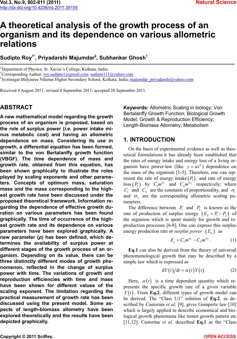
Vol.3, No.9, 802-811 (2011) Natural Science
http://dx.doi.org/10.4236/ns.2011.39105
A theoretical analysis of the growth process of an
organism and its dependence on various allometric
relations
Sudipto Roy1*, Priyadarshi Majumdar2, Subhankar Ghosh1
1Department of Physics, St. Xavier’s College, Kolkata, India;
*Corresponding Author:
2Jyotinagar Bidyasree Niketan Higher Secondary School, Kolkata, India;
Received 8 August 2011; revised 8 September 2011; accepted 28 September 2011.
ABSTRACT
A new mathematical model regarding the growth
process of an organism is proposed, based on
the role of surplus power (i.e. power intake mi-
nus metabolic cost) and having an allometric
dependence on mass. Considering its use in
growth, a differential equation has been formed,
similar to the von Bertalanffy growth function
(VBGF). The time dependence of mass and
growth rate, obtained from this equation, has
been shown graphically to illustrate the roles
played by scaling exponents and other parame-
ters. Concepts of optimum mass, saturation
mass and the mass corresponding to the high-
est growth rate have been discussed under the
proposed theoretical framework. Information re-
garding the dependence of effective growth du-
ration on various parameters has been found
graphically. The time of occurrence of the high-
est growth rate and its dependence on various
parameters have been explored graphically. A
new parameter (ρ) has been defined, which de-
termines the availability of surplus power at
different stages of the growth process of an or-
ganism. Depending on its value, there can be
three distinctly different modes of growth phe-
nomenon, reflected in the change of surplus
power with time. The variations of growth and
reproduction efficiencies with time and mass
have been shown for different values of the
scaling exponent. The limitation regarding the
practical measurement of growth rate has been
discussed using the present model. Some as-
pects of length-biomass allometry have been
explored theoretically and the results have been
depicted graphically.
Keywords: Allometric Scaling in biology; Von
Bertalanffy Growth Function; Biological Growth
Model; Growth & Reproduction Efficiency;
Length-Biomass Allometry; Metabolism
1. INTRODUCTION
On the basis of experimental evidence as well as theo-
retical formulations it has already been established that
the rates of energy intake and energy loss of a living or-
ganism have power-law (like b
y
ax) dependence on
the mass of the organism [1-5]. Therefore, one can rep-
resent the rate of energy intake

1
P and rate of energy
loss


2
P by 1
1
Cm

and 2
2
Cm

respectively; where
1
C and 2 C are the constants of proportionality, and 1

and 2

are the corresponding allometric scaling pa-
rameters.
The difference between 1
P and 2 P is known as the
rate of production of surplus energy

12S
EPP of
the organism which is spent mainly for growth and re-
production processes [6-8]. One can express this surplus
energy production rate or surplus power


S
E as
12
12s
ECm Cm


. (1)
Eq.1 can also be derived from the theory of universal
phenomenological growth that may be described by a
simple law which is expressed as

 
ddYt ttYt  . (2)
Here,


t  is a time dependent quantity which re-
presents the specific growth rate of a given variable


Yt. From Eq.2, different types of growth model can
be derived. The “Class U1” solution of Eq.2, as de-
scribed by Castorina et al. [9], gives Gompertz law [10]
which is largely applied to describe economical and bio-
logical growth phenomena like tumor growth pattern etc
[11,12]. Castorina et al. described Eq.1 as the “Class

S. Roy et al. / Natural Science 3 (2011) 802-811 803
U2” solution of Eq.2 [9].
Over the past few decades, several efforts have been
made to determine the value of two scaling parameters
1

and 2

. In the study of von Bertalanffy, an assump-
tion of 2

= 1 was specified [13,14]. Some studies re-
veal that the metabolic cost is directly proportional to the
mass of an organism, implying 2

= 1 [4,7]. Debates
are still going on over the value of 1

. People attempted
to explain the value of 1

with the help of either meta-
bolic theory of ecology or dynamic energy budget theory.
The metabolic theory of ecology is based on the idea that
the transport of resources takes place through a frac-
tal-like branching network [4,15]. It predicts 1

to be
34, supported by different experimental observations.
The theory of dynamic energy budgets is based on the
concept that the rates of basic physiological processes
are proportional to body surface area, implying
123

 [16,17]. A. R. P. Rau offered an explanation
for the values of scaling parameters, on the basis of
Poiseuille’s law of fluid flow [18]. The chemiosmotic
theory of energy transduction, combined with the method
of quantum statistics, is also applied to explain the varia-
tion in scaling exponents [19]. Many such investigations
show that 123

. In some cases, it may be equal to
34. Vogel showed that biological processes are con-
trolled by different physical processes like convection,
diffusion etc. and the process of mass transport is differ-
ent for different molecules in an organism [20]. da Silva
et al. explained the variation of 1

with the help of
physical processes like diffusion, convection and anoma-
lous diffusion for different organisms [21,22]. According
to the study of Economos [23], the geometry of body
surface, which is different for different organisms, is
related with energy intake of the organism. da Silva et al.
[22] compared the exponent of basal metabolic rates for
different organisms and proposed a theoretical explana-
tion for the different values of that exponent. So, growth
process can be studied using different values of these
scaling exponents.
It has been found through some research [5-7] that, at
the initial stage of growth the surplus power


S
E in-
creases with mass and then it decreases after reaching its
peak value at a mass which is known as the optimum
mass [7]. Based on this fact, we have shown in our ear-
lier studies that 21

  [24,25]. Thus, the scaling ex-
ponent for metabolic cost is found to be greater than the
exponent for energy intake. This is an important conclu-
sion which is also found to be valid according to the
studies of West et al. [26]. In the present article, we have
studied the growth process theoretically, through a model
developed by us on the basis of the relation between
growth rate and surplus power. Using this mathematical
model, an exhaustive analysis of some important aspects
of growth mechanism has been made.
2. MODEL FORMULATION
In the present study, we have taken 21

, under the
consideration that metabolic cost is proportional to the
body volume (which is directly proportional to mass), in
accordance with some studies [3,7,24,27]. Using this
value, Eq.1 is expressed as
1
12s
ECm Cm

. (3)
The above expression of
s
E has been used in all fur-
ther calculations in the present article. Since excess en-
ergy is mainly used for growth and reproduction, these
processes would stop if the surplus power (
s
E) ever be-
comes zero in the life of an organism [7,8]. For a certain
value of m (say h
M
) we have 0
s
E, as evident from
the functional form of
s
E. Using Eq.3, we get

1
11
12h
MCC


. (4)
Apart from the processes of growth and reproduction,
some excess energy is always required for repair and also
to sustain biological processes in situations like sudden
environmental fluctuations etc. According to Kozlowski
[6] and Sebens [7], some surplus energy ()
s
E is always
required for a healthy survival of the organism. There-
fore, taking 0
s
E, Eqs.3 and 4 yield the following
relation

1
11
12 h
mCC M
 
. (5)
Thus, the growth process must stop before reaching
the point where h
mM

. In any growth process, as
t , mass becomes asymptotic to a certain value (say
a
M
) where ah
M
M

. The expression of a
M
, the
highest attainable mass, has been derived later in this
article.
According to some studies [24,25], an organism has a
natural tendency to attain the optimum mass ()
opt
M or
energetic optimum size (EOS), which corresponds to the
greatest surplus power()
s
E [8,12,21]. For
s
E to be
maximum at opt
mM

we must have
1) dd0
s
Em

and 22 2) dd0
s
Em at opt mM

.
The first of the above conditions gives us the follow-
ing expression of optimum mass()
opt
M

1
11
11 2
opt
MCC



. (6A)
Applying the second condition we get
11

. (6B)
Substituting opt mM

in Eq.3 from Eq.6A, the
maximum surplus power (
s
M
E) is obtained as
 
11 1
111
1112 2112 sM
ECCC CCC




. (7)

S. Roy et al. / Natural Science 3 (2011) 802-811 804
The difference between the rates of energy intake and
energetic cost can be termed scope for growth [28] and
energy surplus [29] depending on which energetic costs
are included. If the costs of building gonad are included
then this difference is truly scope for growth. If only the
metabolic maintenance costs are included, this difference
is an energy surplus, used mainly for growth and repro-
duction. Experimental observations suggest that the en-
ergy allocated for reproduction has an allometric de-
pendence on mass [7,21,30]. Therefore, the rate of en-
ergy allocation for reproduction


p
E can be expressed
as
3
3p
ECm

. (8)
where 3

is the allometric scaling exponent and 3 C is
the proportionality constant for the rate of energy spent
for reproduction. Both 3
C and 3

are positive quanti-
ties. In the present study, we have taken 31

, as pro-
posed by Sebens [7]. Using this value, Eq.8 is written as
3p
ECm

(9)
The above expression of
p
E has been used in all
further calculations in this article. The part of the surplus
power (
s
E) which is not used for reproduction, is mainly
used for the growth process. Therefore, the rate of energy
allocation for growth

g
E is given by
1
123
()
gsp
EEECm CCm

  (10)
This energy (
g
E) causes the mass to increase. There-
fore, the rate of variation of mass with time can be ex-
pressed as (with proportionality constant scaled to unity)
1
123
dd( )
g
EmtCmCCm

 (11)
The above equation is similar in form to the von Ber-
talanffy growth function (VBGF), which is basically a
descriptive mechanistic model derived for fish growth
rate, based on a simple mass balance equation [13]. But,
instead of two constants of proportionality, we have three
constants of proportionality to incorporate separately the
effects of energy intake, metabolic cost and reproduction
cost in the growth process.
The growth process continues as long as
g
E remains
non-zero. As the organism reaches the state of maximum
attainable mass (a
M
),
g
E becomes zero. Therefore,
from Eq.11, we obtain
 
1
11
123
,
a
M
CCC CC
 
 (12)
with m = M0 at t = 0, the solution to Eq.11 is given by



1
1
11
1
10
1
1e e
1
tt
mtC CM
C












(13)
Using Eqs.12 and 13 can be expressed as
 

1
11
11
11
0
1e e
tt
a
mt MM









. (14)
From Eq.14 it is found that, as t, a mM. It
means that, after a sufficiently long time, the mass be-
comes almost equal to a
M
. Practically, the organism
does not appear to grow in size when its mass is very
close to a
M
.
Now using Eqs.11 and 13 one may write the growth
rate as

11
11
/1
11
1010
dd
1e ee
g
tt t
mt E
CCMC CM











 


,
(15)
Hence at 0t

, 1
10 0
ddmt CMCM

. This is ac-
tually the initial growth rate and can also be obtained by
putting 0
mM

in Eq.11. We have dd 0mt as
t. Thus, the growth rate never becomes exactly
zero although no growth is practically observed after a
certain age. After reaching the peak value,
g
E de-
creases with time and, at a certain stage, it becomes too
small to be practically measurable. From Eq.11, one can
compute the mass (say
g
M
) for which
g
E has its
highest value. This mass corresponds to the fastest
growth rate and it is expressed as

1
11
11g
MCC



. (16)
Hence, the highest growth rate (
g
M
E) is given by


 
11 1
111
111 11
at
gM gg
EEmM
CC CCC C







. (17)
Comparing
g
M
with opt M in Eq.6A, we get
g
opt
M
M

, since 30C. It clearly implies that an or-
ganism attains the state of fastest growth before reaching
the state of highest surplus power (
s
E).
Eq.13 expresses mass as a function of time. The sur-
plus power (
s
E), being a function of mass, should also
be a function of time. As m approaches its saturation
value (a
M
),
s
E also approaches its saturation value (
s

).
Substituting a mM

in Eq. 3 we get
 
11 1
111
11 21sCCC CCC




. (18)
Depending upon the growth parameters, there can be
three different manners in which growth process can take
place. These three possibilities are discussed below.
CASE 1:
The saturation mass (a
M
) can be smaller than the op-
timum mass (opt
M). This case can be mathematically
described as,

32 11
1
a opt
MM CC

  

. (19)
The growth process, in this case, terminates before

S. Roy et al. / Natural Science 3 (2011) 802-811 805
reaching the state of optimum mass (opt M). The satura-
tion value (
s

) of the surplus power is smaller than
s
M
E.
CASE 2:

32 11
1.
a opt
MM CC

 

(20)
In this case, we have
s
sM
E

 implying that after a
sufficiently long time, the surplus power will almost re-
main at a constant level
s
M
E. As the growth process
terminates the surplus power supply remains constant at
its highest possible value. Therefore, the organism con-
tinues to live with the highest possible rate of surplus
energy production.
CASE 3:

32 11
1.
a opt
MM CC

   

(21)
Here the surplus energy saturates at a mass which ex-
ceeds the optimum mass. Then as like case1 we again
have
s
sM
E

. Here,
s
E initially increases with time
and after reaching the peak value (
s
M
E) it decreases to
its saturation value (
s

).
The conditions expressed by the Eqs.19-21 can be ex-
pressed by a single relation

32 11
1.CC

  

(22)
For the above three cases we have, 1,

 1 and


01

 respectively.
Using Eqs.6A, 12 and 22 we define a quantity R as
 

1
11
11
11
a opt
RMM



 (23)
This ratio (R) is a measure of the saturation mass rela-
tive to optimum mass. Since 11

, we have 1R

for
1

 and 1R for 1

. For 1

, the energy
allocation for growth process continues at most up to the
optimum point. Beyond that point the surplus energy is
allocated mainly for reproduction and other purposes.
For 1

, the energy allocation for growth continues
beyond the optimum point and there is a gradual shift in
energy allocation from growth process to that for repro-
duction. Using Eqs.13 and 22 we get




 
1
1
11
1
112 110
1e1 e
tt
mt
CC M





 

 

,
(24)
where

2
2121 1
11CC



  
.
Using the above expression of time-dependent mass,
the surplus power (
s
E) can be expressed as,


11
1
1
1
1
1
10
11
1
20
1e e
1e e
tt
s
tt
ECA M
CA M


 

 

 

 






(25)
where





112 11
1AC C   and

2
2121 1
11CC



  . Eq.25 shows how
s
E, as a function of time, depends on the value of

.
Let us now define a time period T

as the time re-
quired for the organism to attain a mass m

where
a
mM



and 01


. Applying this definition and
using Eq.14 one may obtain
  





11
11
10
11 ln11
a
TC MM




 .
(26)
In Eq.26, it is evident that as 1

increases, more time
is required to attain a certain fraction (

) of the satura-
tion mass (a
M
). For organisms with higher values of
1

, the growth process continues for a longer time.
In the context of growth, one can define growth effi-
ciency


g

as the ratio of the amount of surplus en-
ergy used for growth to the total surplus energy available
at the moment, and can be expressed as,


11
12312
1.dd
ggs s
EEEmt
CmCCmCmCm

 

(27)
Since dd 0mt as t, we must have 0
g


as t.
In a similar fashion, one can define the reproduction
efficiency


p

as the ratio of the amount of surplus
energy used for reproduction to the total surplus energy
available at the moment, and it can be expressed as

1
31 2
1
pg
Cm CmCm

  . (28)
As t, 0
g

 and therefore 1
p

.
It is consistent with the practical observation that, as
mass increases the proportion of energy allocation for
growth decreases and the energy allocation for reproduc-
tion increases.
The rate of change of growth and reproduction effi-
ciencies with respect to mass can be expressed as


11
2
131 12
dd dd1
pg
mmCCm CmCm

 
(29)
Since 11


, the right hand side of Eq.29 is a posi-
tive quantity. Therefore, as mass increases,
p

contin-
ues to increase and
g

continues to decrease. Eq.29
suggests that, under no circumstances, dd
pm

and
dd
gm

can be equal to zero. As a result one concludes
that an organism, in its life span, never attains a mass for
which its reproduction (or, growth) efficiency would be a
maximum. In different organisms the growth efficiency
seems to have a universal dependence on relative body
mass [31,32]. Using the small amount of available data,
Makarieva et al. [27] has concluded that there is a nega-
tive correlation between growth efficiency and metabolic

S. Roy et al. / Natural Science 3 (2011) 802-811 806
rate. So the conclusion, drawn from Eq.28 is in good
agreement with the literature in this topic.
The time taken by the organism to reach the state of
highest growth rate can be determined by substituting
g
mM in Eq.13 from Eq.16. This span of time, de-
noted by h T is




1
11
11
1
1110 1
111
1
10
ln
ln 11
h
a
TCCCCMCC
MM












 

(30)
A Special Case: Length-Biomass Allometry
In our recent study of length-biomass allometry of bi-
dimensional seaweeds we have shown that the variation
of length with time can be described properly in terms of
two length parameters perpendicular to each other [33].
These are actually the sides of the smallest rectangle that
can enclose the organism. This theoretical analysis was
made in an attempt to explain the experimental findings
of Scrosati on flat seaweeds [34]. According to this
theoretical model, these two length parameters (say L1
and L2 ) has a power-law relation between them. This
relation is given by,

21
LkL

. (31)
Here, k is a constant of proportionality. From experi-
mental observations, an average estimate of

was
found to be 1.119 for the organisms described in our arti-
cle [33]. These length parameters, 1 L and 2 L, have
separate allometric relations with the mass of the organ-
ism. In the present article we have explored the mass-
time relationship. Therefore, one can now formulate the
length-time relationship of such species.
For the species of bi-dimensional seaweeds described
in that article [33], an average estimate of the length-
biomass allometry can be expressed by the following
equations.
0.472
17.811 Lm. (32A)

0.528
21
9.976 LkLkm

 . (32B)
The mass (m) in the above equations is a function of
time and its variation with time is described by the Eqs.
13 and 14 of the present study. It is a common observa-
tion that growth does not take place identically along two
perpendicular directions in any flat organism. From the
above equations the rates of growth along these direc-
tions can be expressed as
0.528
1
dd3.687 ddLtm mt

, (33A)
0.472
2
dd5.267 ddLtkm mt

. (33B)
Here, ddmt is a function of time. Its dependence on
time is expressed by Eq.15 of the present study.
3. GRAPHICAL DEPICTION AND
ANALYSIS
Using the expressions derived in this article, we have
illustrated various growth features graphically.
Figure 1 shows the general nature of dependence of
mass (m) and growth rate (dm/dt) on time. These graphs
are based on the Eqs.13 and 15. The mass initially in-
creases rapidly with time and, after a sufficiently long
time, it becomes asymptotic to the value of a
M
. The
rate of growth (dm/dt) has a very sharp rise at the initial
stage and, after reaching its peak value, it decreases
slowly, becoming negligible after a sufficiently long time.
As t, we have a mM and dd0mt. This
figure shows that the growth process never stops but it
becomes so slow that it does not remain perceptible after
a certain point of time (such as, at nearly t = 5 in Figure
1).
Figure 2 shows the variation of growth rate as a func-
tion of mass for different values of the scaling exponent
1

. For higher values of 1

, the growth rate is higher
and the duration of growth process is longer. At the very
initial stage of growth, the rise in growth rate is almost
independent of 1

. The time required for attaining the
peak rate is longer for higher values of 1

. After reach-
ing the peak value, the growth rate decreases but it does
not fall as rapidly as it rises at the initial stage.
The graphs in Figure 3 show the change of mass of an
organism with time for different values of the constant
1
C. As time goes on, the mass (m) becomes closer and
Figure 1. It shows the variation of mass and growth rate as
functions of time. Here, the mass increases with a gradually
decreasing rate and finally it becomes asymptotic to the value
of Ma. The rate of growth rises fast at the initial stage; reaches
its peak value and then continues to decrease slowly. At
t, we have a mM and dd0mt. In this case the
value of Ma is 1.953. The growth rate reaches its highest value
at m = Mg = 0.579.

S. Roy et al. / Natural Science 3 (2011) 802-811 807
Figure 2. These plots show the change of the growth rate with
mass for different values of the scaling exponent σ1. For higher
values of σ1, the growth process continues for a longer time and
the growth rate becomes higher. At the very initial stage of
growth, the rise in growth rate seems to be almost independent
of σ1. As σ1 increases, the time required for attaining the peak
rate increases. After reaching the peak value, the growth rate
decreases but it does not fall as rapidly as it rises at the initial
stage. The values of Mg for these three cases are 2.370, 5.063
and 10.486.
Figure 3. These plots show how the mass of an organism in-
creases with time for different values of the constant C1. The
mass (m) approaches a saturation level (Ma) which increases
with a rise in C1. After a certain point of time the rise in mass
becomes so slow that practically no growth can be observed.
The values of Ma for these three cases are 1, 3.375 and 8.
closer to its saturation level (Ma) which increases with a
rise in C1. After a long time the mass changes so slowly
than no growth can be practically observed. The values
of Ma for these three cases are 1, 3.375 and 8. These va-
lues are consistent with Eq.12, according to which, Ma
increase as the ratio 1 CC and σ1 become larger.
The graphs in Figure 4 show the dependence of
growth rate on time for different values of the constant
1
C. It is evident from these graphs that the time required
for attaining the peak growth rate is independent of 1
C.
For higher values of this constant, the growth rate is
higher at any stage of the growth process. The change in
mass remains perceptible until dm/d t becomes negligible.
This effective termination point of growth is found to be
the same for the cases shown in this figure and in Figure
3. Therefore, the effective duration of growth process is
independent of 1
C.
Figure 5 shows the dependence of growth rate on time
for different values of the constant C. As C increases, the
growth rate becomes smaller and the effective duration
of growth process becomes shorter. It is found in these
graphs that, as C increases, the time to reach the peak
rate becomes shorter. According to Eqs.13 and 15, as C
increases, the value of

increases and hence the or-
ganism approaches the effective termination point faster.
Figure 6 shows the variation of growth rate with time
for different values of the scaling exponent 1

. For
higher values of 1

, the effective duration of growth
process is longer. At the very early stage of growth, an
organism with smaller value of 1

has greater growth
rate. Apart from this stage, organisms with higher values
of 1

have larger growth rates in general. An organism
with larger value of 1

takes more time in attaining the
peak growth rate.
The variation of surplus power with time, for different
values of the

, is shown in Figure 7. For 1


,
s
E
Figure 4. This figure shows the variation of growth rate with
time for different values of the constant C1. For higher values
of this constant, the growth rate becomes higher at any stage of
the growth process. For these three cases, the growth rates at-
tain their respective peaks at the same time. The increase in
mass remains perceptible up to a certain point where dm/dt is
almost zero. This effective termination point of growth is found
to be the same for the cases shown in this figure. Thus, the
effective duration of growth process is independent of C1.

S. Roy et al. / Natural Science 3 (2011) 802-811 808
Figure 5. These plots show the variation of growth rate with
time for different values of the constant C. For higher values of
this constant, the growth process becomes slower at any stage
of the growth process. It is evident from the graphs that as C
increases, the time required for attaining the peak rate becomes
shorter. The increase in mass remains perceptible up to a cer-
tain point where dm/dt is almost zero. For higher values of C,
the organism approaches this effective termination point with
greater rapidity. Thus, the effective duration of growth process
becomes shorter for higher values of C.
Figure 6. This figure shows the variation of growth rate with
time for different values of the scaling exponent σ1. It is clearly
evident from these graphs that, as σ1 increases, the effective
duration of growth process increases. At the very early stage of
growth, an organism with smaller value of σ1 has greater
growth rate. Except for this very small period, growth rate is
higher for larger values of σ1. For higher values of σ1, the or-
ganism takes more time to attain the state of largest growth
rate.
tends to reach the highest possible surplus power (
s
M
E),
implying that the organism continues to live with the
largest supply of surplus power. For 1

,
s
E initially
increases with time, reaches the peak value at opt mM

and, beyond that point, it attains saturation at a level
Figure 7. This figure shows the variation of surplus power with
time for different values of the constant ρ. For ρ = 1 we have
Ma = Mopt, for ρ < 1 we have Ma > Mopt and for ρ > 1 we have
Ma < Mopt. For ρ = 1, the saturation value of Es is equal to the
highest possible surplus power (EsM). For ρ < 1, Es initially
increases with time, reaching its peak value (EsM) at m = Mopt
and then decreases to saturate at a level smaller than EsM. For ρ
> 1, the mass saturates at a level smaller than Mopt and conse-
quently, Es saturates at a level smaller than EsM.
smaller than
s
M
E. For 1

, the mass attains its satu-
ration level before reaching the value of opt
M and
therefore,
s
E saturates at a level smaller than
s
M
E.
Figure 8 shows the change of growth efficiency (
g

)
and reproduction efficiency (
p

) with respect to the ra-
tio a mM , which is actually a measure of mass relative
to its saturation value. As the growth process proceeds
towards completion, this ratio (a mM ) approaches unity.
This ratio, therefore, is a measure of the degree of com-
pletion of the growth process in an organism. As growth
continues,
g

decreases from 1 to 0 and
p

increases
from 0 to 1. With a rise in mass, the utilization of surplus
energy for reproduction increases and its allocation for
growth decreases.
Figure 9 show the variation of growth efficiency with
time for different values of the constant

. At 0t

,
the efficiency has the highest value (i.e. unity), for any
value of

. The growth efficiency decreases with time
and it approaches its lowest value (i.e. zero) as t,
for any value of

. As

increases, the growth effi-
ciency decreases faster with time. For higher values of

, the growth efficiency is smaller at any stage of the
growth process. Thus, for larger values of

, the utili-
zation of surplus energy for growth is smaller.
Figure 10 shows the variation of T

as a function of

, for different values of the scaling exponent 1

. For
any value of

, T

is larger for higher values of 1

.
Near the right edge of the above frame, a vertical line has
been drawn to mark the point where the mass attains
95% of its saturation level (a
M
). Near this point, the

S. Roy et al. / Natural Science 3 (2011) 802-811 809
Figure 8. This figure shows the variations of growth efficiency
(εg) and reproduction efficiency (εp) with respect to the ratio
m/Ma. As the growth process approaches termination, this ratio
(m/Ma) approaches unity. As growth continues, εg decreases
from 1 to 0 and εp increases from 0 to 1. With a rise in mass,
the utilization of surplus energy for reproduction increases and
its allocation for growth decreases.
Figure 9. These graphs show the variation of growth efficiency
with time for different values of the constant ρ. At t = 0, the
efficiency has the highest value (i.e. unity), irrespective of the
value of ρ. The growth efficiency is found to decrease with
time and it approaches its lowest value (i.e. zero) as t in
all these three cases. As ρ becomes larger, the growth efficiency
falls more rapidly with time. For higher values of ρ, the growth
efficiency is smaller at any stage of the growth process. Thus,
for larger values of ρ, smaller fraction of surplus energy is util-
ized of for growth.
slopes of these curves become extremely high, implying
the fact that a very long time is required for a slight
change in mass. This vertical line almost marks the ef-
fective termination point of growth because any practical
observation (or measurement) of growth becomes more
and more difficult at this stage.
Figure 11 shows the variation of the length parameters
(L1 and L2) of a bi-dimensional organism with time.
These plots are based on the Eqs.32A and B for L1
Figure 10. This figure shows the variation of Tλ as a function
of λ, for different values of the scaling exponent σ1. For any
value of λ, Tλ is larger for higher values of σ1. The vertical line,
near the right edge of the frame, mark the point where m = 0.95
Ma. Very high slope near this point implies that practically very
little rise in mass is observable at this stage of the growth proc-
ess.
Figure 11. This figure shows the variation of the length pa-
rameters (L1 and L2) of bi-dimensional organisms with time.
One of the parameters attains the state of saturation earlier than
the other.
and L2 respectively. Here, the time dependence of mass
(m) has been obtained from Eq.13. One of the parame-
ters attains the state of saturation earlier than the other,
which is quite consistent with our observations.
Figure 12 shows the rate of change of two length pa-
rameters of a bi-dimensional organism as functions of
time. These plots are based on the Eqs.33A and B for L1
and L2 respectively. Here, the time dependence of the
growth rate (ddmt) has been obtained from Eq.15. Any
of these rates attains a maximum value and then de-
creases to zero asymptotically. One of the rates attains
peak value earlier and goes to zero faster than the other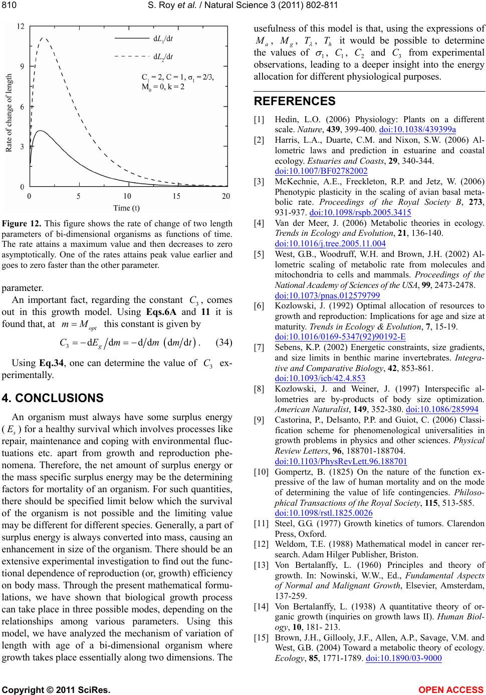

S. Roy et al. / Natural Science 3 (2011) 802-811 810
Figure 12. This figure shows the rate of change of two length
parameters of bi-dimensional organisms as functions of time.
The rate attains a maximum value and then decreases to zero
asymptotically. One of the rates attains peak value earlier and
goes to zero faster than the other parameter.
parameter.
An important fact, regarding the constant 3 C, comes
out in this growth model. Using Eqs.6A and 11 it is
found that, at opt mM this constant is given by

3dd dddd g
CEm mmt . (34)
Using Eq.34, one can determine the value of 3 C ex-
perimentally.
4. CONCLUSIONS
An organism must always have some surplus energy
(
s
E) for a healthy survival which involves processes like
repair, maintenance and coping with environmental fluc-
tuations etc. apart from growth and reproduction phe-
nomena. Therefore, the net amount of surplus energy or
the mass specific surplus energy may be the determining
factors for mortality of an organism. For such quantities,
there should be specified limit below which the survival
of the organism is not possible and the limiting value
may be different for different species. Generally, a part of
surplus energy is always converted into mass, causing an
enhancement in size of the organism. There should be an
extensive experimental investigation to find out the func-
tional dependence of reproduction (or, growth) efficiency
on body mass. Through the present mathematical formu-
lations, we have shown that biological growth process
can take place in three possible modes, depending on the
relationships among various parameters. Using this
model, we have analyzed the mechanism of variation of
length with age of a bi-dimensional organism where
growth takes place essentially along two dimensions. The
usefulness of this model is that, using the expressions of
a
M
,
g
M
, T

, h T it would be possible to determine
the values of 1

, 1 C, 2 C and 3 C from experimental
observations, leading to a deeper insight into the energy
allocation for different physiological purposes.
REFERENCES
[1] Hedin, L.O. (2006) Physiology: Plants on a different
scale. Nature, 439, 399-400. doi:10.1038/439399a
[2] Harris, L.A., Duarte, C.M. and Nixon, S.W. (2006) Al-
lometric laws and prediction in estuarine and coastal
ecology. Estuaries and Coasts, 29, 340-344.
doi:10.1007/BF02782002
[3] McKechnie, A.E., Freckleton, R.P. and Jetz, W. (2006)
Phenotypic plasticity in the scaling of avian basal meta-
bolic rate. Proceedings of the Royal Society B, 273,
931-937. doi:10.1098/rspb.2005.3415
[4] Van der Meer, J. (2006) Metabolic theories in ecology.
Trends in Ecology and Evolution, 21, 136-140.
doi:10.1016/j.tree.2005.11.004
[5] West, G.B., Woodruff, W.H. and Brown, J.H. (2002) Al-
lometric scaling of metabolic rate from molecules and
mitochondria to cells and mammals. Proceedings of the
National Academy of Sciences of the USA, 99, 2473-2478.
doi:10.1073/pnas.012579799
[6] Kozlowski, J. (1992) Optimal allocation of resources to
growth and reproduction: Implications for age and size at
maturity. Trends in Ecology & Evolution, 7, 15-19.
doi:10.1016/0169-5347(92)90192-E
[7] Sebens, K.P. (2002) Energetic constraints, size gradients,
and size limits in benthic marine invertebrates. Integra-
tive and Comparative Biology, 42, 853-861.
doi:10.1093/icb/42.4.853
[8] Kozlowski, J. and Weiner, J. (1997) Interspecific al-
lometries are by-products of body size optimization.
American Naturalist, 149, 352-380. doi:10.1086/285994
[9] Castorina, P., Delsanto, P.P. and Guiot, C. (2006) Classi-
fication scheme for phenomenological universalities in
growth problems in physics and other sciences. Physical
Review Letters, 96, 188701-188704.
doi:10.1103/PhysRevLett.96.188701
[10] Gompertz, B. (1825) On the nature of the function ex-
pressive of the law of human mortality and on the mode
of determining the value of life contingencies. Philoso-
phical Transactions of the Royal Society, 115, 513-585.
doi:10.1098/rstl.1825.0026
[11] Steel, G.G. (1977) Growth kinetics of tumors. Clarendon
Press, Oxford.
[12] Weldom, T.E. (1988) Mathematical model in cancer rer-
search. Adam Hilger Publisher, Briston.
[13] Von Bertalanffy, L. (1960) Principles and theory of
growth. In: Nowinski, W.W., Ed., Fundamental Aspects
of Normal and Malignant Growth, Elsevier, Amsterdam,
137-259.
[14] Von Bertalanffy, L. (1938) A quantitative theory of or-
ganic growth (inquiries on growth laws II). Human Biol-
ogy, 10, 181- 213.
[15] Brown, J.H., Gillooly, J.F., Allen, A.P., Savage, V.M. and
West, G.B. (2004) Toward a metabolic theory of ecology.
Ecology, 85, 1771-1789. doi:10.1890/03-9000

S. Roy et al. / Natural Science 3 (2011) 802-811 811
[16] Kooijman, S.A.L.M. (2010) Dynamic energy budget
theory for metabolic organisation. 3rd Edition, Cam-
bridge University Press, Cambridge.
[17] Sousa, T., Domingos, T. and Kooijman, S.A.L.M. (2008)
From empirical patterns to theory: A formal metabolic
theory of life. Philosophical Transactions of the Royal
Society B, 363, 2453-2464. doi:10.1098/rstb.2007.2230
[18] Rau, A.R.P. (2002) Biological scaling and physics. Jour-
nal of Biosciences, 27, 475-478.
doi:10.1007/BF02705043
[19] Demetrius, L. (2006) The origin of allometric scaling
laws in biology. Journal of Theoretical Biology, 243,
455-467. doi:10.1016/j.jtbi.2006.05.031
[20] Vogel, S. (2004) Living in a physical world. Journal of
Biosciences, 29, 391-397. doi:10.1007/BF02712110
[21] Da Silva, J.K.L. and Barbosa, L.A. (2007) Non-universal
Interspecific Allometric Scaling of Metabolism. Journal
of Physics A, 40, F1-F7.
[22] Da Silva, J.K.L. and Barbosa, L.A. (2009) Non-universal
interspecific allometric scaling of metabolism. Brazilian
Journal of Physics, 39, 699-706.
[23] Economos, A.C. (1982) On the origin of biological simi-
larity. Journal of Theoretical Biology, 94, 25-60.
doi:10.1016/0022-5193(82)90328-9
[24] Biswas, D., Das, S.K. and Roy, S. (2008) Importance of
scaling exponents and other parameters in growth mecha-
nism: An analytical approach. Theory in Biosciences, 127,
271-276. doi:10.1007/s12064-008-0045-9
[25] Biswas, D., Das, S.K. and Roy, S. (200/8) Dependence of
the individual growth process upon allometric scaling
exponents and other parameters. Journal of Biological
Systems, 16, 151-163. doi:10.1142/S0218339008002411
[26] West, G.B., Brown, J.H. and Enquist, B.J. (2004) Growth
model based on first principle or phenomenology. Func-
tional Ecology, 18, 188-196.
d oi:1 0. 1111/ j.0269 -8463.2004.00857.x
[27] Makarieva, A.M., Gorshkov, V.G. and Li, B.-L. (2004)
Ontogenetic growth: Models and theory. Ecological
Modelling, 176, 15-26.
doi:10.1016/j.ecolmodel.2003.09.037
[28] Warren, C.E. and Davis, G.E. (1967) Laboratory studies
on the feeding bioenergetics and growth of fish. In:
Gerking, S.D., Ed., The Biological Basis for Freshwater
Fish Production, Blackwell, Oxford, 175-214.
[29] Sebens, K.P. (1979) The energetics of asexual reproduc-
tion and colony formation in benthic marine invertebrates.
Integrative and Comparative Biology, 19, 683-697.
doi:10.1093/icb/19.3.683
[30] Sebens, K.P. (1982) The limits to indeterminate growth:
An optimal size model applied to passive suspension
feeders. Ecology, 63, 209-222. doi:10.2307/1937045
[31] Pandian, T.J. and Vernberg, F.J. (1987) Animal energetics.
Academic Press, San Diego.
[32] Brody, S. (1945) Biogenetics and growth. Reinhold Pub-
lishing Corporation, New York.
[33] Majumdar, P. and Roy, S. (2010) A theoretical interpreta-
tion of length-biomass allometry of predominantly bidi-
mensional seaweeds. Journal of Theoretical Biology, 266,
226-230.
doi:10.1016/j.jtbi.2010.06.035
[34] Scrosati, R. (2006) Length-biomass allometry in primary
producers: Predominantly bidimensional seaweeds differ
from the ‘‘universal’’ interspecific trend defined by mi-
croalgae and vascular plants. Canadian Journal of Botany,
84, 1159-1166. doi:10.1139/b06-077