Vol.3, No.9, 768-774 (2011) Natural Science
http://dx.doi.org/10.4236/ns.2011.39101
Time and space analysis of two earthquakes in the
Apennines (Italy)
Michele Caputo1,2, Giovanni Sebastiani3,4*
1Physics Department, Sapienza Università di Roma, Roma, Italy;
2Department of Geology and Geophysics, Texas A & M University, College Station, USA;
3Istituto per le Applicazioni del Calcolo “Mauro Picone”, CNR, Roma, Italy;
4Mathematics Department, Sapienza Università di Roma, Roma, Italy; *Corresponding Author:
Received 28 July 2011; revised 30 August 2011; accepted 15 September 2011.
ABSTRACT
In this paper, we study two earthquakes: the
April 6th 2009 earthquake of L’Aquila in the re-
gion of Abruzzo (Italy) and the 1997 Colfiorito
earthquake in the regions of Umbria and Marche
(Italy). The data sets of these two earthquakes
were analysed in both time and space domains.
For time domain we used statistical methods
and models both parametric and non-parametric.
Concerning the space domain, we used Mathe-
matical Morphology filters. The time domain
analysis provides evidence of a possible corre-
lation between seismic activities and the tides of
the crust of the Earth. The results obtained show
evidence that the daily number of earthquakes
of the sequences proceeding and following the
April 6th 2009 earthquake of L’Aquila and that of
the sequence following the 1997 Colfiorito earth-
quake have a periodic component of occurrence
with period of about 7 days. It seems that the
maxima of this component occur at a position of
the Moon with respect to the Earth and the Sun
corresponding to approximately 3 days before
the four main Moon phases. The space domain
analysis indicates that the foreshock activity in
both earthquakes is clustered and concentrated.
Furthermore, in each of the two earthquakes the
clusters are located at about 3 kilometers from
the epicentre of the main shock.
Keywords: Earthquakes; Earth Tides; Periodic
Modeling; Spectral Analysis; Mathematical
Morphology; Foreshocks; Aftershocks
1. INTRODUCTION
In this paper we face two issues. The first concerns the
possibility of detecting the effect of the solid Earth tides
for the triggering of earthquakes, which we approach
with the ansatz that it should be easier to detect the effect
of a small perturbation on a system when the system is
unstable. This condition is verified for both foreshock
and aftershock sequences. The second issue focuses to
contribute to find possible forerunners. To this aim, we
analysed the foreshock activity in space domain.
For many decades, especially to the purpose of predi-
cting earthquakes, it has been speculated that the stress
generated by the solid Earth tides may trigger earth-
quakes. From a theoretical point of view the scientists
generally considered that the stress generated by the tides
in the crust of the Earth could be a direct cause of the
triggering, but this is so small that is seemed unlikely
that it may help triggering the earthquakes in a perfectly
elastic or anelastic Earth crust.
The possibility that solid earth tides may accelerate the
preparation process of the earthquakes and possibly trig-
ger them was first suggested long time ago by Schuster
[1,2]. Since then, a large number of attempts to prove the
correlation between the tides and the occurrence of earth-
quakes have been made and a plethora of papers pub-
lished. A good survey of this literature is in the note of
Métivier et al. [3], who also gave a proof of the existence
of this correlation. In fact, they considered a set of 442,
412 earthquakes and observed a clear correlation be-
tween the phase of the diurnal and semi-diurnal solid
Earth tides and the time of occurrence of earthquakes.
These authors show that the correlation is larger with
shallow earthquakes and that earthquakes occur slightly
more often when the Sun and the Moon are in oppo-
sition.
Atef et al. studied a set of 443,428 earthquakes and
found the existence of two promiment spectral peaks
with periods of one and seven days, respectively [4].
They suggested that the cyclic nature of the cultural
noise level leads to the observed periodicities.

M. Caputo et al. / Natural Science 3 (2011) 768-774 769
For the time domain analysis, we note that the sets of
events which we considered is limited in a central Appe-
nines region with linear length of some tens of kilo-
meters. Therefore, the earthquake events in this region
have approximately the same phase in the Earth tide
effect. The spectral analysis of time series resulting from
the observation of components which have the same fre-
quency and different phases may fail to detect signals of
small amplitude for possible interference. In our case,
due to the limited size of the region where each of the
two earthquakes studied occurred, this problem is irre-
levant.
When considering the statistics of earthquakes occurred
in a very limited region and recorded with modern intru-
mentation, including the smallest observable instrumen-
tally, in order to have a reasonable number of events per
time unit, the number of events is usually counted in
events per day, as done here. We search for possible
periodicities in the daily number of earthquakes proceed-
ing and following the April 6th 2009 earthquake of
L’Aquila in the region of Abruzzo (Italy) and also in the
sequence following the 1997 earthquake of Colfiorito in
the regions of Umbria and Marche (Italy).
We assume that the crust of the Earth, in the seismic
regions, has a large number of small faults with different
orientations [5]. For instance, the faults with area A100
are 5000 times more numerous than those with area A [6].
This is supported by the observations of Wallace in
California [7]. There is therefore a non negligible pro-
bability that the tidal stress field meets a fault with the
appropriate orientation to be effected in the direction to
increase the existing tectonic field. If the stress acting on
this fault is near the value which may trigger an
earthquake then the tidal field may possibly trigger the
earthquake.
2. METHODS OF ANALYSIS
2.1. Time Sequence Analysis
We performed two kinds of analysis of the measured
time sequences: parametric and non-parametric, as des-
cribed below.
Let us first consider the measured foreshock sequence

f
i
M of the number of events happened during each day
i, from day
f
b until day
f
e, within a given spatial
region. This sequence was described here mathematically
by means of a parametric mixture model with an unkown
number of Lorentian components

2
=1
=.
1
p
fk
i
kk
k
C
N
i


 


 (1)
First, we determined the number p of components of
the model. This was done by testing the hypothesis that
there is a significant positive difference of the derivative
discrete approximation
  

 11
2* 2
fff
iii
NNN

 . The
distribution of this quantity under the null hypothesis of
no difference was approximated by the empirical
distribution of the same quantity in a time interval of
days before
f
b, where there is no apparent activity. The
values of the parameters in Eq.1 were found by mini-
mizing the sum of squared differences between the mea-
sured and the theoretical values
 

2
=.
f
f
eff
ii
ib MN

The period of the sequence was estimated here on the
basis of the average difference



11 pp
  be-
tween consecutive peak locations 1kk


,
=1, ,1.kp


The measured sequence

a
i
M of the number of daily
events after the main shock from day a b to day a e
was analysed both parametrically and non-parametrically
to detect the presence of periodicities. In both cases, first
a parametric power-law function was used for modeling
the number of daily events


0
=,
a
i
NCit


 (2)
where 0
t, C and

are real parameters.
Also here the minimization of the sum of squared
differences between

a
i
M and

a
i
N was adopted to
estimate the model parameters. Based on the estimated
model and the measured sequence, their residual diffe-
rence sequence

a
i
R was computed. The residual diffe-
rence sequence was from one side analysed parametri-
cally by modelling

a
i
R as sum of a single component
sinusoidal model and zero mean uncorrelated errors;
amplitude, frequency and phase were estimated by mini-
mizing the sum of squared errors.
The non-parametric analysis of

a
i
R was performed
as follows. In 1987, Jaynes [8] showed that the mode of
the periodogram, i.e. the mode of

C

, time average
of the squared absolute value of the discrete Fourier
transform of a sampled signal, introduced by Schuster
about eighty years before, is a sufficient statistics for the
frequency of a single component periodic signal. Closely
related to the periodogram is the power spectral density
of a stationary stochastic process

Rt , i.e. the Fourier
transform of its autocorrelation function
 
=e d
i
PERtRt



 
 


 (3)
where we assumed that the process auto-correlation fun-
ction only depends on the time lag

, i.e.






=ERtRt

 



. The relation between the pe-
riodogram and the power spectral density is
 
,EC P

  
 (4)
when the time window T goes to. Instead of

M. Caputo et al. / Natural Science 3 (2011) 768-774 770
obtaining the periodogram by calculating the discrete
Fourier transform of data, we have preferred to use the
(sample) power spectral density. This is motivated by the
fact that we could easily cope also with the case where the
residual sequence is modeled by a sum of pure periodic
signals with stochastic amplitudes and phases. Then, to
make consistent the periodogram, it will be sufficient to
weight properly the auto-correlation when calculating its
discrete Fourier transform. The auto-correlation k

at
lag =1, ,=1
aaa
kneb was estimated by


 



=
2
=
=,
eaaaaa
iik
ib
a
keaaa
i
ib
e
RRRR
RR






(5)
where

a
R denotes the sample mean and the sequence
was periodically extended from the original one:
 
=,
aa
i in
a
RR
 (6)
=1,, a in. The power spectral density was then calcu-
lated for a finite number of frequencies by means of the
discrete Fourier transform of the sequence k

,
=1,, a kn.
2.2. Spatial Analysis
Our focus here is to study the distribution of epicentres.
Among the many different approaches available (see e.g.
Caputo and Postpischl 1974, [9]), to have a more rigo-
rous definition of the clustering, we adopted the one of
Mathematical Morphology [10]. This approach was deve-
loped in the applied field of Mineralogy and is based on
topological and algebraic properties of images. In parti-
cular, we used a basic operator, i.e. the opening. This
consists of the application in sequence of first the erosion
operator followed by the one of dilation. We first dis-
cretized the geographical region in a regular lattice


,,,=1,,ij ijm. Let ij N be the total number of
events happened in the cell


,ij within a given time
interval. We reduced the data into binary codes, in which
1 indicates that there is at least one event in the cell and 0
otherwise. Concerning the application of the erosion
operator, given the binary image ij N, a spatial cell that
is qualified 1, is requalified zero when at least one of its
eight neighbouring cells is not qualified 1. Instead, the
dilation operation consists of qualifying 1 the neigh-
bouring cells of each cell qualified 1. The opening opera-
tion produces an image with smooth contours and it elimi-
nates isolated cells qualified 1 or small clusters of them.
3. RESULTS
3.1. Data Description
We analysed two data sets, both recorded by the Isti-
tuto Nazionale Geofisica e Vulcanologia (I.N.G.V.).
The first data set refers to the earthquake in L’Aquila
(Italy) with main shock in 6 April 2009. The sequence of
events corresponds to a spatial region composed by three
circles. The circle centres are the epicentres of the three
events with magnitude larger than 5. These three events
happened in days 6, 7 and 9 April 2009, and the epicen-
tres longitude and latitude were (+13.334, +42.334),
( 13.464,42.275)

 and ( 13.343,42.484) , respecti-
vely. The diameter of the three circles was about 33 km.
We computed the sequence of the daily number of events
happened in the spatial region described above. The first
day was 1 December 2008 and the total number of days
was 298. In Figure 1, the sequence of the daily number
of events is shown. The spatial distribution of the total
number of events in the time interval starting from day
52 to day 80 corresponding to the foreshock activity is
shown in Figure 2. We used a 64 64 lattice of cells
each of about 0.8 km length.
Figure 1. L’Aquila: the daily number of events.
Figure 2. Aquila: the spatial distribution of epicen-
tres during foreshock activity. The image is 64 ×
64 with a pixel length of about 0.8 kilometers. The
North direction is ↑.

M. Caputo et al. / Natural Science 3 (2011) 768-774 771
The second one refers to the earthquake in Colfiorito
(Perugia, Italy) with main activity in September-October
1997. Also here, we computed the sequence of the daily
number of events happened in the spatial region des-
cribed below. The first day was 26 August 1997 and the
total number of days was 81. We analysed a sequence of
events within a circular region with centre the epicentre
of the event with maximum magnitude, that happened in
26 September 1997 and whose longitude and latitude
were ( 12.891,43.023) . The diameter of the circle
was about 50 km. We show the sequence of the daily
number of events in Figure 3. The spatial distribution of
the total number of events in the time interval starting
from day 7 to day 25 corresponding to the foreshock
activity is shown in Figure 4. Also here we used a
64 64 lattice of cells each of about 0.8 km length.
Figure 3. Colfiorito: the daily number of events.
Figure 4. Colfiorito: the spatial distribution of
epicentres during foreshock activity. The image is
64 × 64 with a pixel length of about 0.8 kilo-
meters. The North direction is ↑.
3.2. L’Aquila Earthquake Data Analysis
We first analysed the measured foreshock sequence.
Here the analysis was based on a parametric modeling,
as described in Section 2. The result is shown in Figure
5. In the same figure, the estimated mixture model is
shown. We note the clear presence of four peaks sepa-
rated in average by a time interval of 7.1 days.
We turn now to the analysis of the sequence after the
main shock. This was performed based on either the total
after main shock sequence or a final part of it. In Figure
6, the total after main shock sequence is shown superim-
posed to the power law fitting. The residual difference
between the measured and theoretical sequences is plo-
tted in Figure 7, and its power spectral density is shown
is Figure 8. We note the main peak at a frequency corre-
Figure 5. L’Aquila: the daily number of events in the foreshock
sequence.
Figure 6. L’Aquila: the daily number of events in the after
main shock sequence.

M. Caputo et al. / Natural Science 3 (2011) 768-774 772
Figure 7. L’Aquila: the residual daily number of events in the
after main shock sequence.
Figure 8. L’Aquila: the power spectral density of the residual
daily number of events in the after main shock sequence.
sponding to a period of 7.1 days. The procedure was also
applied to a final part of the after main shock sequence.
The difference between the measured and the theoretical
sequences appears in Figure 9 superimposed to a fitting
by a pure sinusoidal parametric model. The period of the
estimated sinusoidal model was 7.1 days. The non-para-
metric analysis of the residual sequence in Figure 9, by
means of the power spectral density is shown is Figure
10. The maximum peak noted in the last figure corre-
sponds to a period of 7.1 days. We note that the optimi-
zation of the main peak intensity of the power spectral
density with respect to perturbations of the location of
the last sequence datum, corresponded to a sequence
length of 49 days, which a multiple of seven.
We note that the peaks in the foreshock sequence of
Figure 5 correspond to Fridays, while those in the after-
Figure 9. L’Aquila: the residual daily number of events in a
final part of the after main shock sequence.
Figure 10. L’Aquila: the power spectral density of the residual
daily number of events in a final part of the after main shock
sequence.
shock of Figure 9 are located on Sundays. Furthermore,
the corresponding position of the Moon with respect to
the Earth and the Sun was approximately 3 days before
the four main Moon phases (data from US Naval Obser-
vatory, Astronomical Application Department).
We show now the results of the spatial analysis. We
recall Figure 2, where the total counts of events in the
foreshock period from day 52 to day 80 is shown. In Fi-
gure 11, we represent the counts ij N only in the cells
where the Mathematical Morphology opened image is
qualified 1. The image clearly shows the presence of two
clusters close to each other with a maximum linear di-
mension of the largest one of about 5 Kilometers. The
isolated pixel we also put in the figure corresponds to the
epicentre of the main shock. We notice that this epicentre

M. Caputo et al. / Natural Science 3 (2011) 768-774 773
Figure 11. Aquila: the spatial distribution of epicentres during
foreshock activity after the application of Mathematical Mor-
phology filtering. The image is 64 × 64 with a pixel length of
about 0.8 kilometers. The North direction is ↑.
Figure 12. Colfiorito: the residual daily number of events in a
final part of the after main shock sequence.
is about 3 kilometers from the closest cluster.
3.3. Colfiorito Earthquake Data Analysis
Also here, we adopted a power-law model for the after
main shock sequence starting from the relevant shock at
day 51. The difference between the measured and the
theoretical sequences is plotted in Figure 12 superim-
posed to a pure sinusoidal model fit. The period of the
estimated sinusoidal model is 6.7 days. The result of the
non-parametric analysis by the power spectral density is
shown is Figure 13. Here, it is evident a peak at a fre-
quency corresponding to a period of 7.0 days. The opti-
mization with respect to the location of the last datum as
before now corresponds to a a sequence length of 28
days, which again is a multiple of seven.
We note that the peaks in the aftershock of Figure 13
are located on Mondays. Also here, the corresponding
position of the Moon with respect to the Earth and the
Sun was approximately 3 days before the four main Moon
phases (data from US Naval Observatory, Astronomical
Application Department).
Figure 14, shows the counts ij N only in the cells
where the Mathematical Morphology opened image is
qualified 1. The image clearly shows the presence of one
Figure 13. Colfiorito: the power spectral density of the residual
daily number of events in a final part of the after main shock
sequence.
Figure 14. Colfiorito: the spatial distribution of epi-
centres during foreshock activity after the applica-
tion of Mathematical Morphology filtering. The image
is 64 × 64 with a pixel length of about 0.8 kilo-
meters. The North direction is ↑.

M. Caputo et al. / Natural Science 3 (2011) 768-774 774
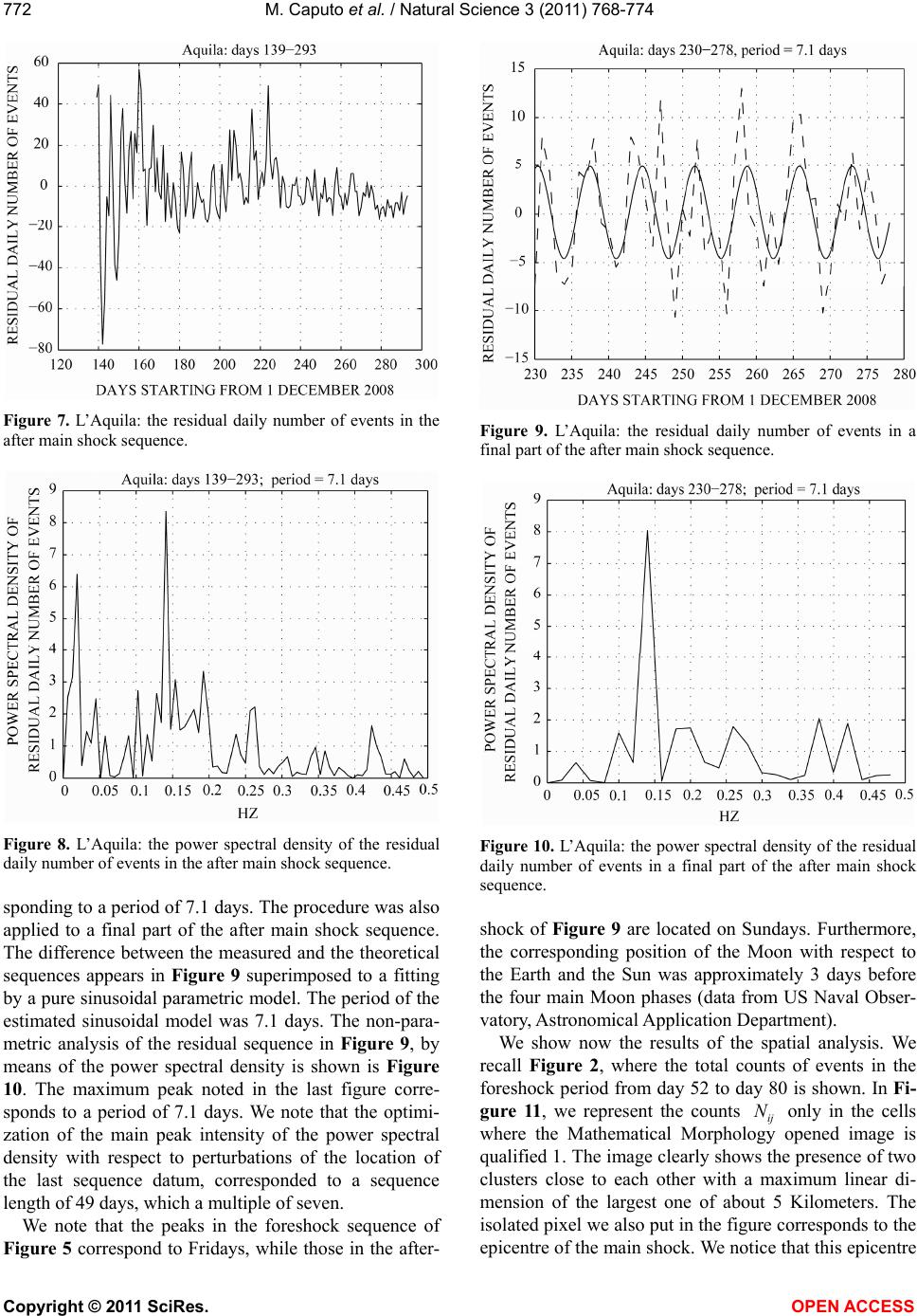
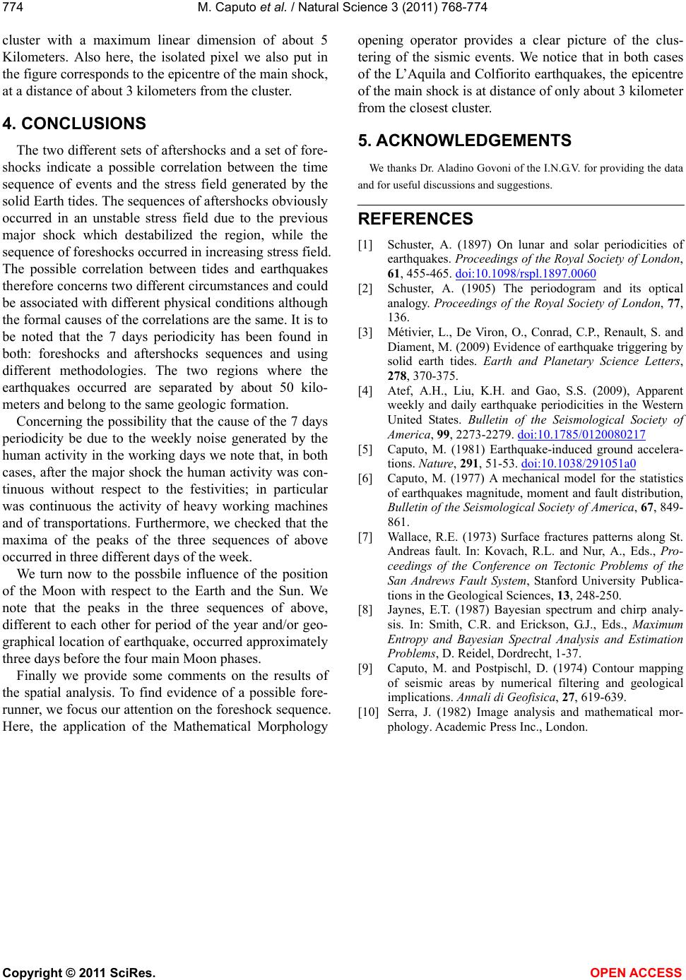
cluster with a maximum linear dimension of about 5
Kilometers. Also here, the isolated pixel we also put in
the figure corresponds to the epicentre of the main shock,
at a distance of about 3 kilometers from the cluster.
4. CONCLUSIONS
The two different sets of aftershocks and a set of fore-
shocks indicate a possible correlation between the time
sequence of events and the stress field generated by the
solid Earth tides. The sequences of aftershocks obviously
occurred in an unstable stress field due to the previous
major shock which destabilized the region, while the
sequence of foreshocks occurred in increasing stress field.
The possible correlation between tides and earthquakes
therefore concerns two different circumstances and could
be associated with different physical conditions although
the formal causes of the correlations are the same. It is to
be noted that the 7 days periodicity has been found in
both: foreshocks and aftershocks sequences and using
different methodologies. The two regions where the
earthquakes occurred are separated by about 50 kilo-
meters and belong to the same geologic formation.
Concerning the possibility that the cause of the 7 days
periodicity be due to the weekly noise generated by the
human activity in the working days we note that, in both
cases, after the major shock the human activity was con-
tinuous without respect to the festivities; in particular
was continuous the activity of heavy working machines
and of transportations. Furthermore, we checked that the
maxima of the peaks of the three sequences of above
occurred in three different days of the week.
We turn now to the possbile influence of the position
of the Moon with respect to the Earth and the Sun. We
note that the peaks in the three sequences of above,
different to each other for period of the year and/or geo-
graphical location of earthquake, occurred approximately
three days before the four main Moon phases.
Finally we provide some comments on the results of
the spatial analysis. To find evidence of a possible fore-
runner, we focus our attention on the foreshock sequence.
Here, the application of the Mathematical Morphology
opening operator provides a clear picture of the clus-
tering of the sismic events. We notice that in both cases
of the L’Aquila and Colfiorito earthquakes, the epicentre
of the main shock is at distance of only about 3 kilometer
from the closest cluster.
5. ACKNOWLEDGEMENTS
We thanks Dr. Aladino Govoni of the I.N.G.V. for providing the data
and for useful discussions and suggestions.
REFERENCES
[1] Schuster, A. (1897) On lunar and solar periodicities of
earthquakes. Proceedings of the Royal Society of London,
61, 455-465. doi:10.1098/rspl.1897.0060
[2] Schuster, A. (1905) The periodogram and its optical
analogy. Proceedings of the Royal Society of London, 77,
136.
[3] Métivier, L., De Viron, O., Conrad, C.P., Renault, S. and
Diament, M. (2009) Evidence of earthquake triggering by
solid earth tides. Earth and Planetary Science Letters,
278, 370-375.
[4] Atef, A.H., Liu, K.H. and Gao, S.S. (2009), Apparent
weekly and daily earthquake periodicities in the Western
United States. Bulletin of the Seismological Society of
America, 99, 2273-2279. doi:10.1785/0120080217
[5] Caputo, M. (1981) Earthquake-induced ground accelera-
tions. Nature, 291, 51-53. doi:10.1038/291051a0
[6] Caputo, M. (1977) A mechanical model for the statistics
of earthquakes magnitude, moment and fault distribution,
Bulletin of the Seismological Society of America, 67, 849-
861.
[7] Wallace, R.E. (1973) Surface fractures patterns along St.
Andreas fault. In: Kovach, R.L. and Nur, A., Eds., Pro-
ceedings of the Conference on Tectonic Problems of the
San Andrews Fault System, Stanford University Publica-
tions in the Geological Sciences, 13, 248-250.
[8] Jaynes, E.T. (1987) Bayesian spectrum and chirp analy-
sis. In: Smith, C.R. and Erickson, G.J., Eds., Maximum
Entropy and Bayesian Spectral Analysis and Estimation
Problems, D. Reidel, Dordrecht, 1-37.
[9] Caputo, M. and Postpischl, D. (1974) Contour mapping
of seismic areas by numerical filtering and geological
implications. Annali di Geofisica, 27, 619-639.
[10] Serra, J. (1982) Image analysis and mathematical mor-
phology. Academic Press Inc., London.