Energy and Power En gi neering, 2011, 3, 565-573
doi:10.4236/epe.2011.34070 Published Online September 2011 (http://www.SciRP.org/journal/epe)
Copyright © 2011 SciRes. EPE
Wind Tunnel at LABINTHAP (Updated)
Rosas Quiterio Pedro, Toledo Velázquez Miguel, Tolentino Eslava Guilibaldo,
Tolentino Eslava René, Sánchez Silva Florencio, Abugaber Francis Juan
Researching and Graduate Section, Applied Hydraulics and Thermal Engineering Laboratory,
Professional Unit Adolfo López Mateos”, Col. Lindavista, México, D.F.
E-mail: mtv49@yahoo.com
Received June 29, 2011; revised July 29, 2011; accepted August 13, 2011
Abstract
Flow behavior in the Thermal Engineering and Applied Hydraulics Laboratory (LABINTHAP) wind tunnel
was investigated by measuring the velocity profiles, turbulence intensity and wall effects with a hot wire
anemometer. Measurements were carried out under wind speeds 5, 15 and 30 m/s in planes located at 1.8, 2.6
and 3.4 m from flow inlet to the test section. The flow showed a good quality with a velocity variation less
than 1%, turbulence intensity lower than 4% and the wall effects allow having an excellent work area in the
test section for the velocities evaluated.
Keywords: Wind Tunnel, Calibration, Measurement, Boundary Layer, Hot Wire Anemometer
1. Introduction
The original LABINTHAP wind tunnel configuration
from National Polytechnic Institute (IPN) is shown in
Figure 1. The wind tunnel was put into service in 1990;
it has not had the capability to be used for accurate
measurements due to the flow uniformity and high tur-
bulence intensity in the test section. First works con-
ducted in this facility were flow visualization [1], bound-
ary layer measurement in different geometries and tur-
bomachinery investigation.
This facility is an open circuit wind tunnel with a suc-
tion and pressure test section. The airflow is generated
by a centrifugal fan driven by a 74.6 kW electrical motor
controlled by a variable frequency drives, to get different
velocities in both test sections. The highest wind velocity
in the suction test section is 75 m/s. This velocity de-
pends on environmental temperature, pressure and hu-
midity registered while tests were being carried out.
The test section has a rectangular cross section of 0.8
m by 0.6 m, a variable length of 5.0 m. The flow inlet
was a bellmouth designed in accordance to AMCA stan-
dards (AMCA 1987), before and after this device there
were two screens to reduce the velocity fluctuation in the
test section.
Recent flow measurement in the low speed wind tun-
nel demonstrated that the velocity variations in the test
section were about 2% and the turbulence intensity was
6.5% [2], this parameters showed the poor quality of the
facility. The Laboratory has undertaken to modify the
wind tunnel to improve the flow quality in the test sec-
tion and get accurate measurements.
The modifications carried out were the design of a
contraction nozzle with an area ratio of 9, five stainless
Figure 1. Original wind tunnel c onfigur ation.
R. Q. PEDRO ET AL.
566
steel screens, a honeycomb and a bellmouth at the begin-
ning of the settling chamber, as can be seen in [1]. The
aim of this work is to present the modifications of the
wind tunnel and, the preliminary flow evaluation of the
LABINTHAP wind tunnel with the contraction nozzle
only by means of velocity and turbulence profiles and,
effect walls.
2. Methodology
2.1. Wind Tunnel Modifications
Modifications proposed to improve flow quality in the
wind tunnel test section are in accordance with the pa-
pers developed by Bradshaw P. and Pankhurst R. C.,
1964 [3] and Metha R. D. and Bradshaw P., 1979 [4].
2.2. Screens and Honeycombs
Screens objectives are reducing the velocity fluctuations
in axial direction and making the velocity profile more
uniform by a static pressure drop. Reference [3] sug-
gested use four screens with an open area ratio of β >
0.57 and the distance between screens have to be of 500
dw (wire diameters). Reference [4] suggested that the
distance between the last screen and the contraction inlet
has to be about 0.2 diameters of the settling chamber.
According to previous criterions, five stainless steel
screens of 20 meshes will be installed in the wind tunnel
settling chamber, wire diameter of 0.23 mm and an open
area ratio of 0.67. The distance between the last screen
and the contraction will be of 500 mm and, the separa-
tions between screens will be of 120 mm (521 dw).
Honeycombs are effective to remove swirl and lateral
mean velocity variations, as long as the flow yaw angles
are not greater than 10˚ [5]. The design parameters for
honeycomb are length to diameter ratio and porosity. The
cell length should be about 6 to 8 times its diameter, as
mentioned in [4]. The honeycomb that will be installed
in the wind tunnel settling chamber will have a cell
size of 10.5 mm, thickness of 0.2 mm and a length of 85
mm.
2.3. Contraction Nozzle and Bellmouth
The purposes of contraction nozzle are: a) to increase the
mean velocity, b) to reduce velocity variations and c) to
reduce velocity fluctuations. The recommended area ra-
tios of the contraction nozzle to get these criterions are 6
to 9, as mentioned in [4]. The method used to design the
contraction nozzle was the one suggested by Morel T.,
1977 [6], this method considered an incompressible and
no viscous flow. The Morel method use two cubic equa-
tions to get the contraction nozzle, both curves are joined
in a point xm.
The principal criterions to design the contraction noz-
zle by this method are: 1) flow uniformity in the exit
nozzle, 2) avoiding flow separation, 3) less contraction
length and 4) minimum boundary layer thickness. To
avoid flow separation pressure coefficient should be 0.42
at the inlet (Cpi) and 0.1 at the contraction exit (Cpo).
These coefficient values let to have a velocity variations
profiles less than 2%.
The contraction design has a contraction area ratio of
9:1, a length of 1680 mm. This area ratio was chosen due
to the laboratory space conditions. The joint of the cubic
equations that form the contraction profiles is xm =
0.531. At inlet of the settling chamber there is a bell-
mounth with a radius of 0.125 of the equivalent diameter
of this device (290 mm).
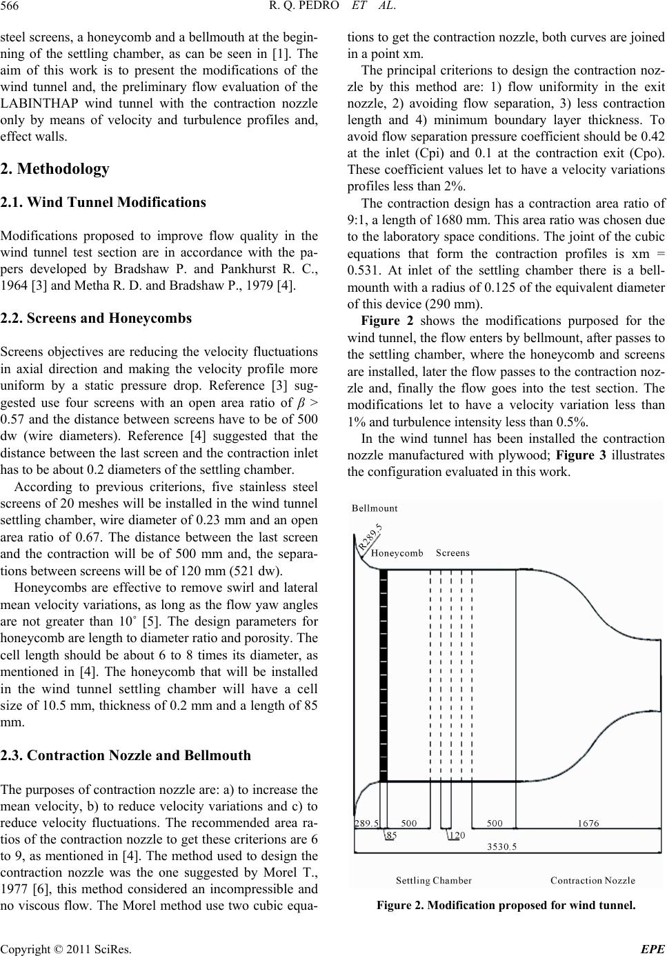
Figure 2 shows the modifications purposed for the
wind tunnel, the flow enters by bellmount, after passes to
the settling chamber, where the honeycomb and screens
are installed, later the flow passes to the contraction noz-
zle and, finally the flow goes into the test section. The
modifications let to have a velocity variation less than
1% and turbulence intensity less than 0.5%.
In the wind tunnel has been installed the contraction
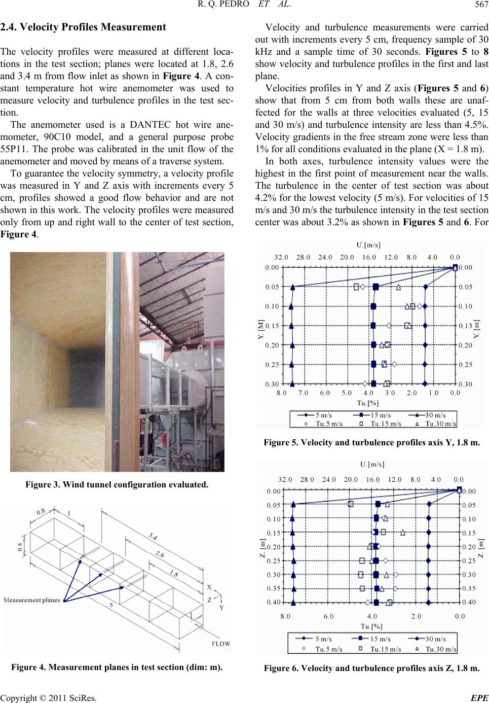
nozzle manufactured with plywood; Figure 3 illustrates
the configuration evaluated in this work.
Figure 2. Modification proposed for wind tunnel.
Copyright © 2011 SciRes. EPE
R. Q. PEDRO ET AL.567
2.4. Velocity Profiles Measurement
The velocity profiles were measured at different loca-
tions in the test section; planes were located at 1.8, 2.6
and 3.4 m from flow inlet as shown in Figure 4. A con-
stant temperature hot wire anemometer was used to
measure velocity and turbulence profiles in the test sec-
tion.
The anemometer used is a DANTEC hot wire ane-
mometer, 90C10 model, and a general purpose probe
55P11. The probe was calibrated in the unit flow of the
anemometer and moved by means of a traverse system.
To guarantee the velocity symmetry, a velocity profile
was measured in Y and Z axis with increments every 5
cm, profiles showed a good flow behavior and are not
shown in this work. The velocity profiles were measured
only from up and right wall to the center of test section,
Figure 4.
Figure 3. Wind tunnel configuration evaluated.
Figure 4. Measurement planes in test section (dim: m).
Velocity and turbulence measurements were carried
out with increments every 5 cm, frequency sample of 30
kHz and a sample time of 30 seconds. Figures 5 to 8
show velocity and turbulence profiles in the first and last
plane.
Velocities profiles in Y and Z axis (Figures 5 and 6)
show that from 5 cm from both walls these are unaf-
fected for the walls at three velocities evaluated (5, 15
and 30 m/s) and turbulence intensity are less than 4.5%.
Velocity gradients in the free stream zone were less than
1% for all conditions evaluated in the plane (X = 1.8 m).
In both axes, turbulence intensity values were the
highest in the first point of measurement near the walls.
The turbulence in the center of test section was about
4.2% for the lowest velocity (5 m/s). For velocities of 15
m/s and 30 m/s the turbulence intensity in the test section
center was about 3.2% as shown in Figures 5 and 6. For
Figure 5. Velocity and turbulence profiles axis Y, 1.8 m.
Figure 6. Velocity and turbulence profiles axis Z, 1.8 m.
Copyright © 2011 SciRes. EPE
R. Q. PEDRO ET AL.
568
the velocity of 15 m/s the turbulence intensity is about
5% from 25 to 35 cm from right wall, Figure 6.
In last measurement plane (X = 3.4 m), the free stream
velocity is reached at 15 cm from the up wall for 30 m/s.
For velocities of 15 m/s and 5 m/s, free stream velocities
are gotten at 10 cm from the wall, Figure 7. Velocity
variation in the free stream zone is less than 1%. Turbu-
lence intensity is about 10% in the first point (5 cm from
the wall) and turbulence intensity in the center of test
section is less than 3.5%.
Velocity profiles illustrate the wall effects at 30 m/s in
this condition the free stream is gotten at 15 cm from the
wall, at 15 m/s is gotten at 10 cm from wall and, at low-
est velocity is gotten at 5 cm. The velocity uniformity is
less than 1% in the free stream zone, Figure 8.
Figure 7. Velocity and turbulence profiles axis Y, 3.4 m.
Figure 8. Velocity and turbulence profiles axis Z, 3.4 m.
Figure 8 shows high turbulence intensity in measure-
ments near right wall (7%) at three velocity conditions
evaluated. For all velocities turbulence intensity is less
than 4% in the free stream zone. Turbulence intensity in
test section center is less than 3% as Figure 8 shows.
Velocities profiles (Figures 5 to 8) show a good flow
quality but turbulence intensity is higher, because the set
up evaluated only had the contraction nozzle at inlet of
flow to the test section. To reduce turbulence and im-
prove velocity uniformity in the test section it is neces-
sary to install the settling chamber and the bellmouth.
2.5. Wall Effects in the Test Section
Wall effects were investigated by measuring the velocity
every 5 mm up to 200 mm from wall. Measurements
were carried out with 55P15 probe and are presented in
Figures 9 and 10.
Frequency and time sample were similar to velocity
and turbulence measurement. Wall effects were measured
at three planes and velocities evaluated. In this paper
Figure 9. Wall effects in X = 3.4 m, axis Y.
Figure 10. Wall effects in X = 3.4 m, axe Z.
Copyright © 2011 SciRes. EPE
R. Q. PEDRO ET AL.569
only the results in axis Y and Z at 3.4 m from flow inlet
to test section are shown. From wall effects measurement
boundary layer thickness was obtained in upper and right
walls for all conditions evaluated, Table 1.
Figure 9 shows that free stream velocity in axis Y is
gotten at 0.075 m, 0.065 m and 0.045 m for 30 m/s, 15
m/s and 5 m/s respectively. Figure 10 presents the wall
effects in Z axe; free stream velocity is gotten at 0.07 m
(30 m/s), 0.06 m (15 m/s) and 0.05 m. (5 m/s) from right
wall. The velocity variations in the free stream zone are
less than 2% for all conditions measured.
From wall effects measurements, it is observed that
turbulence intensity is higher in the measurements from
0.0 m to 0.08 m, in axis Y and Z, and has values from
12% to 16%. Turbulence reduces its value to free stream
zone where it is less than 4.5% for all conditions evalu-
ated.
Velocity profiles and effects in walls measurements in
the low speed wind tunnel section allow to establish the
work section in a range from 5 m/s to 30 m/s in the three
planes evaluated.
2.6. Work Window in Test Section
The boundary layer thickness gotten from wall effects
measurement allow to obtain the work section dimen-
sions for all velocity conditions in the three planes
evaluated. In this work only the development of work
section in the tree planes for highest velocity evaluated
(30 m/s) is presented. Figure 11 shows the work win-
dow for this condition.
Boundary layer thickness gotten in up and right walls
were considered symmetric for the down and left walls.
The previous assumption let to have the work section
dimensions for 30 m/s, in the first plane (1.8 m) the di-
mensions are 0.52 m by 0.69 m; at 2.6 m from flow inlet
free stream zone is 0.47 m by 0.68 m; and in the last
plane located at 3.4 m from nozzle exit is 0.45 m by 0.66
as shown in Figure 11. The atmospheric pressure is a
function of the altitude. In accordance with the definition
of static pressure, the following differential equation is
obtained.
To carry out the characterization of the test section
LABINTHAP lower speed wind tunnel test section in
Table 1. Test section boundary layer thickne ss.
U = 5.5 m/s U = 15.3 m/s U = 30.7 m/s
X[m]
δY[mm] δZ[mm] δY[mm] δZ[mm] δY[mm] δZ[mm]
1.8 25 35 35 45 40 55
2.6 35 45 55 50 65 60
3.4 45 50 65 60 75 70
function of the aforementioned parameters, were perfo-
med a series of measurements with a hot wire anemome-
ter, to determine: frequency f, sample time tand y num-
ber of samples N, for speeds of 5 m/s, 10 m/s, 15 m/s, 20
m/s, 25 m/s and 30 m/s. Measurements were made in the
center of the wind tunnel test section at a distance of 1.6
m to the start of the test section looking for turbulence
levels, frequencies and optimal sampling times. To ob-
tain these measurements it was used a general purpose
probe 55P11 mark.
In Figures 12 and 13 it shows that the turbulence is
stabilized as from the 15 kHz and the sampling time be-
comes unstable after 50 s for the critical speed 5 m/s and
30 m/s, whereby it was established that the optimal sam-
pling frequency for the development of the experimental
phase of this work was 30 kHz and a sampling time of 30
s, so it was obtained a sample of 900,000 data for each
punctual speed measurement was made.
Figure 11. Work section at 30 m/s in X = 3.4 m.
1510 15 20 30 40 50 60 5
20
40
60
0
0.5
1
1.5
2
2.5
3
% Tu
f (kHz)
t (s)
f - t - Tu
0-0.5 0.5-1 1-1.51.5-2 2-2.52.5-3
Figure 12. Turbulence at different frequencies and sam-
pling time of 5 m/s.
Copyright © 2011 SciRes. EPE
R. Q. PEDRO ET AL.
570
According to experimental approaches, the first part of
the characterization was carried out by measuring the
velocity profiles at X = 0.8 m, X = 1.6 m X = 2.4 m for
speeds of 5 m/s, 10 m/s, 15 m/s, 20 m/s, 25 m/s and 30
m/s in the Y and Z axes, making a sweep every 0.05 m
on the axes mentioned. Figures 14-16 shows the velocity
profiles measured with hot wire anemometer at X = 0.8
m, X = 1.6 m, X = 2.4 m respectively.
According to experimental approaches, the second part
of the characterization was carried out by measuring the
boundary layer at X = 0.8 m, X = 1.6 m X = 2.4 m for
speeds of 5 m / s, 10 m / s, 15 m / s, 20 m / s, 25 m / s
and 30 m / s in the Y and Z axes, making a sweep in each
of these axes 0.05 m.
Figures 17-19 shows the velocity profiles obtained
with hot wire anemometer X = 0.8 m, X = 1.6 m, X = 2.4
m respectively. To determine the velocity profiles a
boundary layer probe 55P15, Dantec was used.
151015 20 30 40 50 60 5
20
40
60
0
0.2
0.4
0.6
0.8
1
1.2
1.4
% Tu
f (kHz)
t (s)
f - t - Tu
0-0.2 0.2-0.40.4-0.6 0.6-0.8 0.8-11-1.2 1.2-1.4
Figure 13. Velocity profiles.
Figure 14. Velocity profiles in the Z axis in the plane of 0.8
m.
Figure 15. Velocity profiles in the Z axis in the plane of 1.6 m.
Figure 16. Velocity profiles in the Z axis in the plane of 2.4 m.
Figure 17. Boundary layer in the X axis, in the plane at 0.8 m.
2.7. Turbulence
According to experimental approaches, the third part of
the charaterization was carried out by measuring the
level of turbulence in X = 0.8 m, X = 1.6 m, X = 2.4 m
for the range of speed from 5 m/s to 30 m/s in the center
of the calibration zone.
The Figure 20 shows the turbulence levels obtained
with the hot wire anemometer X = 1.6 m. To determine
Copyright © 2011 SciRes. EPE
R. Q. PEDRO ET AL.571
Figure 18. Boundary layer in the X axis, in the plane at 1.6 m.
Figure 19. Boundary layer in the X axis, in the plane at 2.4 m.
U vs TU
0
0.1
0.2
0.3
0.4
0.5
0.6
0.7
0.8
0.9
1
0510 15 2025 30
m/s
%TU
TU-ATU-B TU-C
Figure 20. Turbulence against speed.
the velocity profiles it was used a general purpose probe
55P11, Dantec brand, which was placed with its support
parallel to the flow, leaving the sensor perpendicular to
the main flow and as close as possible to the wall.
2.8. Flow in Corners
According to experimental methodology, the final part of
the characterization was carried out by measuring the
flow in corners at 0.8 m, 1.6 m and 2.4 m for the range of
speed from 5 m/s to 30 m/s as shown in Figure 21.
To carry out the measurement of flow in the corners it
was realized a sweep in the Y and Z axes, simultaneously.
The sweep was divided into two cross sections, the first
at each 0.03 m in those axes.
3. Analysis of Results
This chapter shows the analysis of results of this work, in
which were made the measurements of velocity profiles,
boundary layer thickness, and flow turbulence level in
corners, all in order to determine the area calibration.
3.1. Speed Profiles
About velocity profiles, we can conclude that the level of
fluctuation in the profiles decreased satisfactorily, as can
be seen in Figures 22 and 23, corresponding to the Z and
Y axes and Tables 2 and 3, respectively.
3.2. Turbulence
In the turbulence intensity can conclude that fulfilled one
of the main objectives of this work, which was to reduce
the level of turbulence (Table 4) to reach the level of
turbulence required by CENAM. In Figure 24 we can
Figure 21. Corner flow in the plane at 2.4 m.
Copyright © 2011 SciRes. EPE
R. Q. PEDRO ET AL.
572
Figure 22. Boundary Layers on the X axis in the plane at
0.8 m.
Figure 23. Boundary Layers on the X axis in the plane at
0.8 m.
Table 2. Uniformity of speed profiles before and after
changes in X = 1.6 m.
AFTER BEFORE AFTER BEFORE AFTER BEFORE
Z U5 U
5 U
15 U
15 U
30 U
30
(m) (m/s) (m/s) (m/s) (m/s) (m/s) (m/s)
0 0 0 0 0 0 0
0.15 5.021 5.5815 15.0715.2275 25.02 30.2545
0.2 5.059 5.6475 15.0715.1365 25.046 30.1615
0.25 5.065 5.654 15.09415.1835 25.015 30.1405
0.3 5.068 5.6155 14.94915.204 24.884 30.1475
0.35 5.059 5.652 14.97915.142 24.854 30.074
0.4 5.064 5.6455 14.92615.122 25.024 30.1405
U (%) 5.6 13.2667 1.46673.5967 0.7167 5.3033
Table 3. Uniformity of speed profiles before and after
changes in X = 1.6 m.
AFTER BEFORE AFTER BEFORE AFTER BEFORE
Y U5 U
5 U
15 U
15 U
30 U
30
(m) (m/s) (m/s) (m/s) (m/s) (m/s) (m/s)
0 0 0 0 0 0 0
0.15 5.175 5.6165 15.01515.2245 30.011 29.9775
0.2 5.058 5.6025 15.07615.1615 30.067 29.9975
0.25 5.11 5.5885 14.93815.1675 29.987 30.0235
0.3 5.107 5.6455 15.04415.122 30 30.1405
U (%) 1.25 11.325 1.825 1.8875 1.625 3.475
Table 4. Turbulence at different velocities and different
distances X = 1.6.
U Tu
(%)
(m/s)
AFTER BEFORE
5 0.679 3.2
10 0.699 3.2
15 0.639 4
20 0.717 3.4
25 0.679 3.5
30 0.727 3.5
Figure 24. Boundary Layers on the X axis in the plane at
0.8 m.
see the change in the level of turbulence before and after
the proposed changes.
We can also note that the sampling time is decreased
by 75% for speeds of 5 m/s to 25 m/s as well as the sam-
pling rate from 900,000 to 100,000 data, as shown in
Figure 25.
Despite this, we have the equation of the Nyquist theo-
rem, which by definition indicates that the sample size
should be the square of the wavelength at which the sen-
sor operates.
In Figure 26 it is clear that the level of turbulence has
been reduced to less than 1%, so LABINTHAP tunnel is
at the level of those who are in countries like Japan,
Germany, France, Brazil and USA.
The modifications carried out were the design of a con-
traction nozzle with an area ratio of 9, five stainless steel
screens, a honeycomb and a bellmouth at the beginning
of the settling chamber, as can be seen in [2]. The
Copyright © 2011 SciRes. EPE
R. Q. PEDRO ET AL.
Copyright © 2011 SciRes. EPE
573
1510 15 20 3040 50 60 5
20
40
60
0
1
2
3
4
5
6
7
8
9
10
% Tu
f (kHz)
t (s)
f - t - Tu
0-11-22-33-44-5 5-6 6-7 7-8 8-9 9-10
aim of this work is to present the modifications of the
wind tunnel and, the preliminary flow evaluation of the
LABINTHAP wind tunnel with the contraction nozzle
only by means of velocity and turbulence profiles and,
effect walls.
4. Conclusions
The low speed wind tunnel test section at LABINTHAP
was evaluated by mean of velocity and turbulence pro-
files, and wall effects for velocities of 5, 15 and 30 m/s
in planes located at 1.8, 2.6 and 3.4 m from flow inlet to
test section. This is the first evaluation with only the
contraction nozzle installed in the test section.
Velocity variations in the free stream inside test sec-
tion were less than 1% and turbulence intensity was less
than 4.0% for all conditions evaluated. The contraction
nozzles reduce the turbulence intensity from 6.5% (ori-
ginal configuration) to 4.0%. Nowadays screens and
honeycomb are installed to reduce turbulence intensity
and improve flow quality in the test section.
(a)
1510 152030 40 50 60 5
20
40
60
0
1
2
3
4
5
6
7
8
9
10
% Tu
f (kHz)
t (s)
f - t - Tu
0-1 1-2 2-3 3-4 4-5 5-6 6-7 7-8 8-9 9-10
Modifications shown in this work reduce turbulence
intensity to less than 0.5% and improve the velocity dis-
tribution inside the test section. This allows to do re-
search in fluid dynamics, turbomachinery, boundary layer
and airspeed metrology.
5. References
[1] G. Tolentino, M. Toledo and V. Zurita, “Experimental
Study of Boundary Layer on a NACA 65-010 Blade Us-
ing Some Flow Visualization Techniques. Flow Visuali-
zation and Imagine Processing of Multiphase System,”
Proceeding of the 1995 ASME/JSME Fluids Engineering
Division Conference, South Carolina, 13-18 August 1995.
[2] E. R. Tolentino, V. M. Toledo, E. G. Tolentino and S. F.
Sánchez, “Modificaciones al Túnel de Viento del
LABINTHAP para Mediciones de Velocidad de Aire
desde 5 m/s hasta 30 m/s,” Simposio de Metrología 2004,
Querétaro, 25-27 October 2004.
(b)
Figure 25. (a) Boundary Layers on the X axis in the plane at
0.8 m. (b). Boundary Layers on the X axis in the plane at
0.8 m.
[3] P. Bradshaw and R. C. Pankhurst, “The Design of Low
Speed Wind Tunnels,” Progress in Aeronautical Sci-
ences, Vol. 5, 1964, pp. 1-69.
[4] R. D. Metha and P. Bradshaw, “Desing Rules for Small
Low Speed Wind Tunnels,” Aeronautical Journal of the
Royal Aeronautical Society, Vol. 73, 1979, pp. 443-449.
[5] J. B. Barlow, W. H. Rae and A. Pope, “Low Speed Wind
Tunnel Testing,” 3rd Edition, John Wiley and Sons, Ho-
boken, 1999.
[6] T. Morel, “Design of Two-Dimensional Wind Tunnel
Contractions,” Journal of Fluids Engineering, Vol. 99,
No. 2, 1977, pp. 371-378.
http://dx.doi.org/10.1115/1.3448764
Figure 26. Turbulence level.