Paper Menu >>
Journal Menu >>
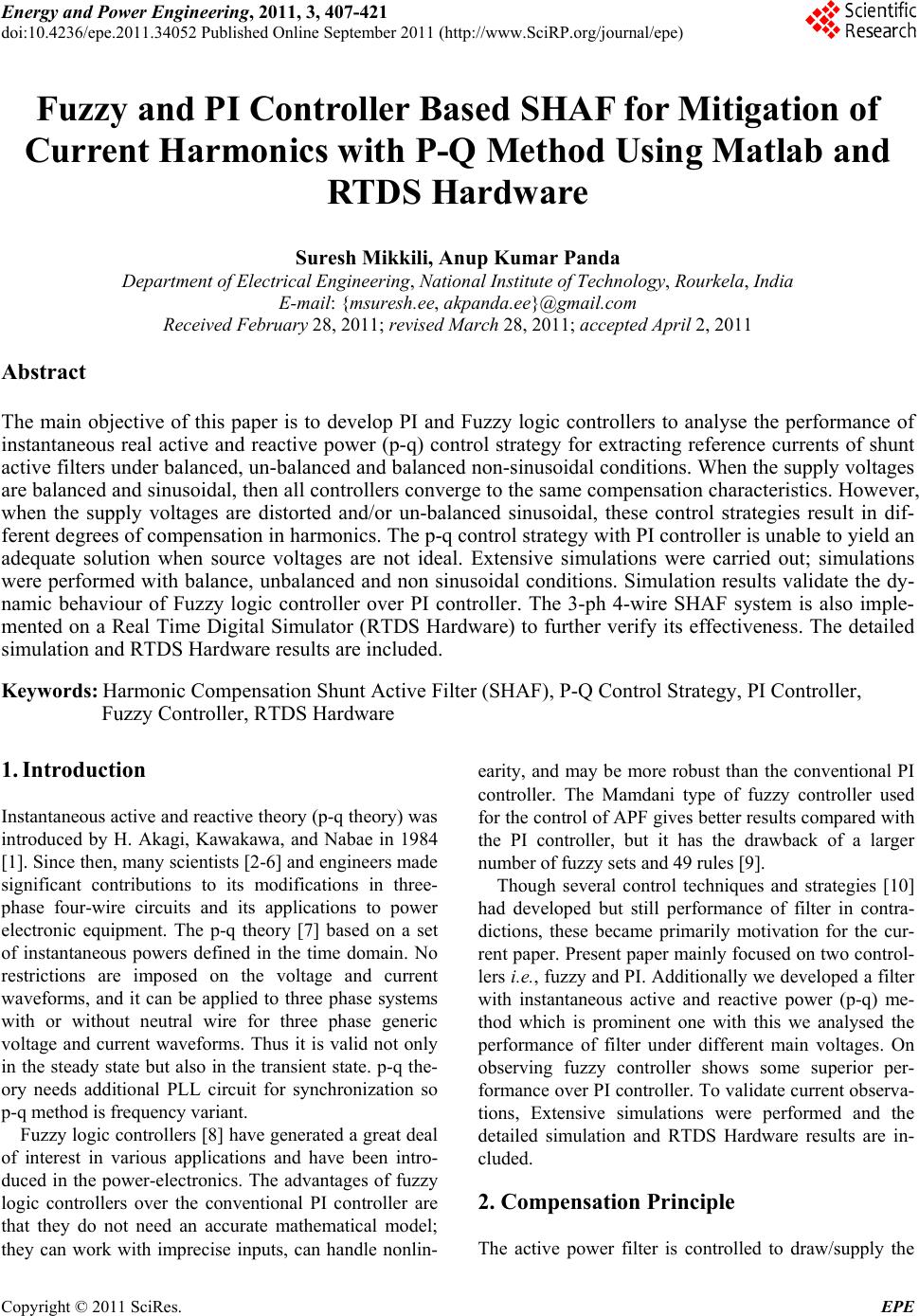 Energy and Power En gi neering, 2011, 3, 407-421 doi:10.4236/epe.2011.34052 Published Online September 2011 (http://www.SciRP.org/journal/epe) Copyright © 2011 SciRes. EPE Fuzzy and PI Controller Based SHAF for Mitigation of Current Harmonics with P-Q Method Using Matlab and RTDS Hardware Suresh Mikkili, Anup Kumar Panda Department of Electrical Engineering, National Institute of Technology, Rourkela, India E-mail: {msuresh.ee, akpanda.ee}@gmail.com Received February 28, 2011; revised March 28, 2011; accepted April 2, 2011 Abstract The main objective of this paper is to develop PI and Fuzzy logic controllers to analyse the performance of instantaneous real active and reactive power (p-q) control strategy for extracting reference currents of shunt active filters under balanced, un-balanced and balanced non-sinusoidal conditions. When the supply voltages are balanced and sinusoidal, then all controllers converge to the same compensation characteristics. However, when the supply voltages are distorted and/or un-balanced sinusoidal, these control strategies result in dif- ferent degrees of compensation in harmonics. The p-q control strategy with PI controller is unable to yield an adequate solution when source voltages are not ideal. Extensive simulations were carried out; simulations were performed with balance, unbalanced and non sinusoidal conditions. Simulation results validate the dy- namic behaviour of Fuzzy logic controller over PI controller. The 3-ph 4-wire SHAF system is also imple- mented on a Real Time Digital Simulator (RTDS Hardware) to further verify its effectiveness. The detailed simulation and RTDS Hardware results are included. Keywords: Harmonic Compensation Shunt Active Filter (SHAF), P-Q Control Strategy, PI Controller, Fuzzy Controller, RTDS Hardware 1. Introduction Instantaneous active and reactive theory (p-q theory) was introduced by H. Akagi, Kawakawa, and Nabae in 1984 [1]. Since then, many scientists [2-6] and engineers made significant contributions to its modifications in three- phase four-wire circuits and its applications to power electronic equipment. The p-q theory [7] based on a set of instantaneous powers defined in the time domain. No restrictions are imposed on the voltage and current waveforms, and it can be applied to three phase systems with or without neutral wire for three phase generic voltage and current waveforms. Thus it is valid not only in the steady state but also in the transient state. p-q the- ory needs additional PLL circuit for synchronization so p-q method is frequency variant. Fuzzy logic controllers [8] have generated a great deal of interest in various applications and have been intro- duced in the power-electronics. The advantages of fuzzy logic controllers over the conventional PI controller are that they do not need an accurate mathematical model; they can work with imprecise inputs, can handle nonlin- earity, and may be more robust than the conventional PI controller. The Mamdani type of fuzzy controller used for the control of APF gives better results compared with the PI controller, but it has the drawback of a larger number of fuzzy sets and 49 rules [9]. Though several control techniques and strategies [10] had developed but still performance of filter in contra- dictions, these became primarily motivation for the cur- rent paper. Present paper mainly focused on two control- lers i.e., fuzzy and PI. Additionally we developed a filter with instantaneous active and reactive power (p-q) me- thod which is prominent one with this we analysed the performance of filter under different main voltages. On observing fuzzy controller shows some superior per- formance over PI controller. To validate current observa- tions, Extensive simulations were performed and the detailed simulation and RTDS Hardware results are in- cluded. 2. Compensation Principle The active power filter is controlled to draw/supply the 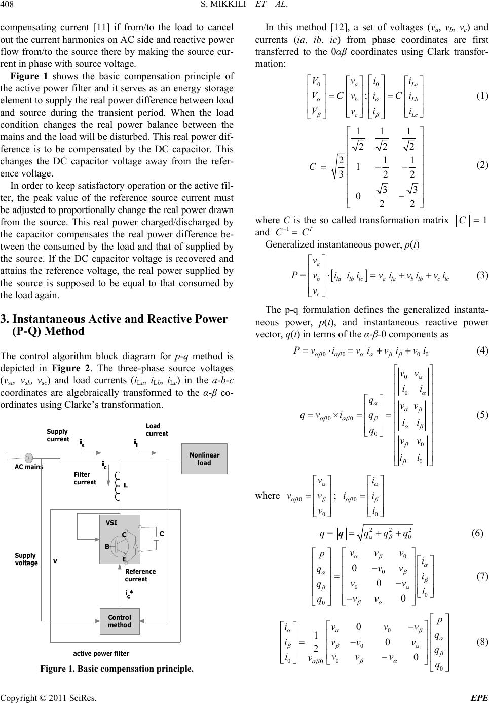 S. MIKKILI ET AL. 408 compensating current [11] if from/to the load to cancel out the current harmonics on AC side and reactive power flow from/to the source there by making the source cur- rent in phase with source voltage. Figure 1 shows the basic compensation principle of the active power filter and it serves as an energy storage element to supply the real power difference between load and source during the transient period. When the load condition changes the real power balance between the mains and the load will be disturbed. This real power dif- ference is to be compensated by the DC capacitor. This changes the DC capacitor voltage away from the refer- ence voltage. In order to keep satisfactory operation or the active fil- ter, the peak value of the reference source current must be adjusted to proportionally change the real power drawn from the source. This real power charged/discharged by the capacitor compensates the real power difference be- tween the consumed by the load and that of supplied by the source. If the DC capacitor voltage is recovered and attains the reference voltage, the real power supplied by the source is supposed to be equal to that consumed by the load again. 3. Instantaneous Active an d Reactive Power (P-Q) Method The control algorithm block diagram for p-q method is depicted in Figure 2. The three-phase source voltages (vsa, vsb, vsc) and load currents (iLa, iLb, iLc) in the a-b-c coordinates are algebraically transformed to the α-β co- ordinates using Clarke’s transformation. Figure 1. Basic compensation principle. In this method [12], a set of voltages (va, vb, vc) and currents (ia, ib, ic) from phase coordinates are first transferred to the 0αβ coordinates using Clark transfor- mation: 00 ; aL b cL Vvii VC viC i Vvii a Lb c (1) 11 1 22 2 21 1 32 33 022 C 1 2 (2) where C is the so called transformation matrix 1C and 1T C C Generalized instantaneous power, p(t) a blalblcalab lbc lc c v P= vi iiv ivivi v 0 (3) The p-q formulation defines the generalized instanta- neous power, p(t), and instantaneous reactive power vector, q(t) in terms of the α-β-0 components as 00 0 Pviv iv iv i (4) 0 0 00 0 0 0 v v i i qv v qvi q i i q v v i i (5) where 0 0 v v v v ; 0 0 i i i i 222 0 q= qqq q (6) 0 0 0 0 0 0 0 0 vvv pi vv qi vv qi vv q (7) 0 0 00 0 0 0 10 20 p iv vv q i vv vq iv v v vq (8) Copyright © 2011 SciRes. EPE  S. MIKKILI ET AL. Copyright © 2011 SciRes. EPE 409 αβ α β βα v vi p i qv -v a α b β c 11v 1 V22 33 V0 - v 22 2v 3 L a α L b L c 11 1 - - 22 33 0 - 22 i i2i i3i * cααβ c * cββα c αβ i*v v-P 1 =22 i*v -vq v+v cα c 1 0 i* ca i* 13 2 i*= cb i* 322 i* cc 13 - 22 Figure 2. Control method for Shunt current compensation based on p-q theory. where 0 . In the new coordinates sys- tem, the instantaneous power has two components: the zero-sequence instantaneous real power, P0, and the in- stantaneous real power due to positive and negative se- quence components, 222 0 vvvv P 2 0 22 00 sref LL sref sref v iPP i v vv i (14) 4. Construction of PI Controller 0 Pt Pt Pt (9) 0 Pt vi00 (10) Figures 3 and 4 show the internal structure of the control circuit. The control scheme consists of PI controller, lim- iter, and three phase sine wave generator for reference current generation and generation of switching signals. The peak value of reference currents is estimated by regulating the DC link voltage. The actual capacitor voltage is compared with a set reference value [13]. v Pt ii v i v i v (11) Using the above equations and considering the or- thogonal nature of vectors v and 0qv q the re- ference source current in the αβ0 frame is 0 0 000 0 0 10 2 0 s s s p v v v iq i v v vq iv v v v q (12) The objective of the p-q strategy is to get the source to give only the constant active power demanded by the load 0sL L Pt Pt Pt In addition, the source must deliver no zero-sequence active power 0 (so that the zero-sequence com- ponent of the voltage at the PCC does not contribute to the source power). The reference source current in the α-β-0frame is therefore 0 sref i 0 0 0 0 00 10 22 0 00 0 LL sref sref sref PP ivvv i vvv i vv vv (13) The error signal is then processed through a PI con- troller, which contributes to zero steady error in tracking the reference current signal. The output of the PI con- troller is considered as peak value of the supply current (Imax), which is composed of two components: 1) funda- mental active power component of load current, and 2) loss component of APF; to maintain the average capaci- tor voltage to a constant value. Peak value of the current (Imax) so obtained, is multiplied by the unit sine vectors in phase with the respective source voltages to obtain the reference compensating currents. These estimated refer- ence currents (Isa*, Isb*, Isc*) and sensed actual currents (Isa, Isb, Isc) are compared at a hysteresis band, which gives the error signal for the modulation technique. This error signal decides the operation of the converter switches. In this current control circuit configuration, the source/supply currents Isabc are made to follow the sinu- soidal reference current Iabc, within a fixed hysteretic band. The width of hysteresis window determines the ource current pattern, its harmonic spectrum and the s  S. MIKKILI ET AL. Copyright © 2011 SciRes. EPE 410 loss P p 0 p Figure 3. Reference current extraction with conventional p-q method with PI controller. Figure 4. Conventional PI controller. switching frequency of the devices. The DC link capacitor voltage is kept constant thr- oughout the operating range of the converter. In this scheme, each phase of the converter is controlled inde- pendently. To increase the current of a particular phase, the lower switch of the converter associated with that particular phase is turned on while to decrease the cur- rent the upper switch of the respective converter phase is turned on. With this one can realize, potential and feasi- bility of PI controller. 5. Construction of Fuzzy Logic Controller Figure 5 shows the internal structure of the control cir- cuit. The control scheme consists of Fuzzy controller [14], limiter, and three phase sine wave generator for reference current generation and generation of switching signals. The peak value of reference currents is estimated by regulating the DC link voltage. The actual capacitor voltage is compared with a set reference value. The error signal is then processed through a Fuzzy controller, which contributes to zero steady error in tracking the reference current signal. A fuzzy controller converts a linguistic control strat- egy into an automatic control strategy, and fuzzy rules are constructed by expert experience or knowledge data- base [15]. Firstly, input Error E and change in Error have been placed of the angular velocity to be the input vari- ables of the fuzzy logic controller. Then the output vari- able of the fuzzy logic controller is presented by the con- trol Current Imax . To convert these numerical variables into linguistic variables, the following seven fuzzy levels or sets are chosen as: NB (negative big), NM (negative medium), NS (negative small), ZE (zero), PS (positive small), PM (positive medium), and PB (positive big) as shown in Figure 6. Table 1. Rule base. (de/dt)/e NB NMNS Z PS PMPB NB NB NB NB NB NM NS Z NM NB NB NB NM NS Z PS NS NB NB NM NS Z PS PM Z NB NMNS Z PS PMPB PS NMNS Z PS PM PB PB PM NS Z PS PM PB PB PB PB Z PS PM PB PB PB PB  S. MIKKILI ET AL. Copyright © 2011 SciRes. EPE 411 Figure 5. Proposed fuzzy inference system. (a) (b) I max μ(I max ) (c) Figure 6. (a) Input variable “E” membership function. (b) Input change in error normalized MF. (c) Output Imax normalized MF.  S. MIKKILI ET AL. Copyright © 2011 SciRes. EPE 412 The fuzzy controller is characterized as follows: 1) Seven fuzzy sets for each input and output. 2) Fuzzification using continuous universe of dis- course. 3) Implication using Mamdani’s “min” operator. 4) De-fuzzification using the “centroid” method. The bock diagram of Fuzzy logic controller is shown in Figure 7. It consists of blocks Fuzzification Interface. Knowledge base. Decision making logic. Defuzzification. 6. RTDS Hardware This simulator was developed with the aim of meeting the transient simulation needs of electromechanical drives and electric systems while solving the limitations of tra- ditional real-time simulators which is shown in Figure 8. It is based on a central principle: the use of widely avail- able, user-friendly, highly competitive commercial pro- ducts (PC platform, Simulink™). The real-time simulator [16] consists of two main tools: a real-time distributed simulation package (RT-LAB) for the execution of Simulink block diagrams on a PC-cluster, and algo- rithmic toolboxes designed for the fixed-time-step simu- lation of stiff electric circuits and their controllers. Real- time simulation and Hardware-In-the-Loop (HIL) appli- cations are increasingly recognized as essential tools for engineering design and especially in power electronics and electrical systems. 6.1. Simulator Architecture 6.1.1. Block Diagram and Schematic Interface The present real-time electric simulator is based on RT LAB real-time, distributed simulation platform; it is op- timized to run Simulink in real-time, with efficient fixed- step solvers, on PC Cluster. Based on COTS non-pro- prietary PC components, RT LAB [17] is a modular real-time simulation platform, for the automatic imple- mentation of system-level, block diagram models, on standard PC’s. It uses the popular MATLAB/Simulink as a front-end for editing and viewing graphic models in block-diagram format. The block diagram models be- come the source from which code can be automatically generated, manipulated and downloaded onto target pro- cessors (Pentium and Pentium-compatible) for real-time or distributed simulation. 6.1.2. Simula t or Co nfiguration In a typical configuration (Figure 9), the RT-LAB simu- lator consists of One or more target PC’s (computation nodes); one of the PCs (Master) manages the communication be- tween the hosts and the targets and the communica- tion between all other target PC’s. The targets use the REDHAT real-time operating system. Figure 7. Block diagram of fuzzy logic controller (FLC).  S. MIKKILI ET AL.413 Figure 8. RT-LAB simulator architecture. Figure 9. RTDS hardware. One or more host PC’s allowing multiple users to access the targets; one of the hosts has the full control of the simulator, while other hosts, in read-only mode, can receive and display signals from the real-time simulator. I/O’s of various types (analog in and out, digital in and out, PWM in and out, timers, encoders, etc.). I/O’s can be managed by dedicated processors dis- tributed over several nodes. 7. Simulation and RTDS Results Figures 10-12 illustrates the performance of shunt active power filter under different main voltages, as load is highly inductive, current draw by load is integrated with rich harmonics. Figure 10 illustrates the performance of Shunt active power filter under balanced sinusoidal voltage condition, THD for p-q method with PI Controller using Matlab simulation is 2.15% and using RTDS Hard ware is 2.21%; THD for p-q method with Fuzzy Controller using Matlab simulation is 1.27% and using RTDS Hard ware is 1.45%. Figure 11 illustrates the performance of Shunt active power filter under un-balanced sinusoidal voltage condi- ion, THD for p-q method with PI Controller using Matlab t Copyright © 2011 SciRes. EPE  S. MIKKILI ET AL. Copyright © 2011 SciRes. EPE 414 0.352 0.354 0.356 0.3580.360.362 0.364 0.366 0.3680.370.372 -400 -300 -200 -100 0 100 200 300 400 Time (Sec) Source Voltage (Volts) 0.352 0.354 0.356 0.3580.360.362 0.364 0.366 0.3680.370.372 -150 -100 -50 0 50 100 150 Time (Sec) Source Current (Amps) 0.352 0.354 0.356 0.3580.360.362 0.364 0.366 0.3680.370.372 -150 -100 -50 0 50 100 150 Time (Amps) Filter Current (Amps) 0.352 0.354 0.356 0.3580.360.362 0.364 0.366 0.3680.37 0.372 0 200 400 600 800 1000 Time (Sec) DC Link Voltage (Volts) 0.352 0.354 0.356 0.358 0.36 0.3620.364 0.3660.3680.370.372 -40 -30 -20 -10 0 10 20 30 40 Time (Sec) Load Current (Amps) 010 2030 40 50 0 0.2 0.4 0.6 0.8 1 Harmonic order 3ph 4w Bal Sin p-q with PI Controller ( MATLAB Simulation)3ph 4w Bal Sin p-q with PI Controller ( RT DS Hardware) THD= 2.15% Mag (% of Fundamental) (a) (b)  S. MIKKILI ET AL.415 0.352 0.354 0.356 0.3580.36 0.362 0.364 0.366 0.368 0.370.372 -400 -300 -200 -100 0 100 200 300 400 Time (Sec) Source Voltage (Volts) 0.352 0.354 0.356 0.3580.36 0.362 0.3640.366 0.368 0.37 0.372 -150 -100 -50 0 50 100 150 Time (Sec) Source Current (Amps) 0.352 0.354 0.356 0.3580.36 0.362 0.3640.366 0.368 0.37 0.372 -150 -100 -50 0 50 100 150 Time (Sec) Filter Current (Amps) 0.3520.354 0.3560.3580.360.3620.364 0.3660.3680.370.372 0 200 400 600 800 1000 DC Link Voltage (Volts) Time (Sec) 3ph 4w Bal Sin p-q with Fuzzy Controller (MATLAB Simulation) 0.352 0.354 0.356 0.3580.360.362 0.364 0.366 0.3680.370.372 -40 -30 -20 -10 0 10 20 30 40 Time (Sec) Load Current (Amps) 010 2030 4050 0 0.2 0.4 0.6 0.8 1 Harmonic order 3ph 4w Bal Sin p-q with Fuzzy Controller (RTDS Hardware) THD= 1.27% Mag (% of Fundamental) (c) (d) Figure 10. 3ph 4w ire shunt ative filter response wi th p-q control strate gy under balanced sinusoidal usi ng. (a) P I wi th matlab; (b) PI with RTDS hardware; (c) Fuzzy with matlab; (d) Fuzzy with RTDS hardware. Copyright © 2011 SciRes. EPE  S. MIKKILI ET AL. 416 0.352 0.354 0.356 0.3580.360.362 0.364 0.366 0.3680.370.372 -400 -300 -200 -100 0 100 200 300 400 Time (Sec) Source Voltage (Volts) 0.352 0.354 0.3560.3580.360.362 0.364 0.366 0.3680.370.372 -150 -100 -50 0 50 100 150 Time (Sec) Source Current (Amps) 0.352 0.354 0.356 0.3580.360.362 0.364 0.3660.3680.370.372 -150 -100 -50 0 50 100 150 Time (Sec) Filter Current (Amps) 0.352 0.354 0.356 0.3580.360.362 0.364 0.366 0.3680.370.372 0 200 400 600 800 1000 Time (Sec) DC Link Voltage (Volts) 0.352 0.354 0.356 0.3580.360.362 0.364 0.366 0.3680.370.372 -40 -30 -20 -10 0 10 20 30 40 Time (Sec) Load Current (Amps) 010 2030 40 50 0 1 2 3 4 5 Harmonic order 3ph 4w Un-bal Sin p-q with PI Controller ( MATLAB Simulation) 3ph 4w Un-bal Sin p-q with PI Controller ( RT DS Hardware) THD= 4. 16% Mag (% of Fundamental) (a) (b) Copyright © 2011 SciRes. EPE  S. MIKKILI ET AL.417 0.3520.354 0.356 0.3580.360.362 0.364 0.366 0.3680.37 0.372 -400 -300 -200 -100 0 100 200 300 400 Time (Sec) Source Voltage (Volts) 0.3520.354 0.356 0.3580.360.362 0.364 0.366 0.3680.37 0.372 -150 -100 -50 0 50 100 150 Time (Sec) Source Current (Amps) 0.352 0.354 0.356 0.3580.36 0.3620.364 0.366 0.3680.37 0.372 -150 -100 -50 0 50 100 150 Time (Sec) Filter Current (Amps) 0.3520.354 0.356 0.3580.360.362 0.364 0.366 0.3680.37 0.372 0 200 400 600 800 1000 Time (Sec) DC Link Voltage (Volts) 0.352 0.354 0.356 0.3580.36 0.3620.364 0.366 0.3680.37 0.372 -40 -30 -20 -10 0 10 20 30 40 Time (Sec) Load Current (Amps) 010 20 30 4050 0 0.2 0.4 0.6 0.8 1 Harmonic order 3ph 4w Un-bal Sin p-q with Fuzzy Controller 3ph 4w Un-bal Sin p-q with Fuzzy Controller ( MATLAB Simulation)( RT DS Hardware) THD= 2.98% Mag (% of Fundamental) (c) (d) Figure 11. 3-ph 4wire shunt ative filter response with p-q control strategy under un-balanced sinusoidal using. (a) PI with Matlab; (b) PI with RTDS hardware; (c) Fuzzy with matlab; (d) Fuzzy with RTDS hardware. Copyright © 2011 SciRes. EPE  S. MIKKILI ET AL. 418 0.352 0.354 0.356 0.3580.360.3620.364 0.3660.368 0.37 0.372 -400 -300 -200 -100 0 100 200 300 400 Time (Sec) Source Voltage (Volts) 0.352 0.354 0.356 0.3580.360.3620.364 0.3660.368 0.37 0.372 -150 -100 -50 0 50 100 150 Time (Sec) Source Current (Amps) 0.352 0.354 0.356 0.3580.360.3620.364 0.3660.368 0.37 0.372 -150 -100 -50 0 50 100 150 Time (Sec) Filter Current (Amps) 0.352 0.354 0.356 0.3580.360.3620.364 0.3660.368 0.37 0.372 0 200 400 600 800 1000 Time (Sec) DC Link Voltage (Volts) 0.352 0.354 0.356 0.3580.360.362 0.364 0.3660.3680.370.372 -40 -30 -20 -10 0 10 20 30 40 Time (Sec) Load Current (Amps) 010 20 3040 50 0 2 4 6 8 10 Harmonic order 3ph 4w Non-Sin p-q with PI Controller ( MATLAB Simulation) 3ph 4w Non-Sin p-q with PI Controller ( RT DS Hardware) THD= 5.31% Mag (% of Fundamental) (a) (b) Copyright © 2011 SciRes. EPE  S. MIKKILI ET AL.419 3ph 4w Non-Sin p-q with Fuzzy Controller ( MATLAB Simulation) 0.3520.354 0.3560.3580.36 0.362 0.364 0.3660.368 0.370.372 -400 -300 -200 -100 0 100 200 300 400 Time (Sec) Source Voltage (Volts) 0.3520.354 0.356 0.3580.36 0.362 0.364 0.3660.368 0.370.372 -150 -100 -50 0 50 100 150 Time (Sec) Source Current (Amps) 0.3520.354 0.3560.3580.36 0.362 0.364 0.3660.368 0.370.372 -150 -100 -50 0 50 100 150 Time (Sec) Filter Current (Amps) 0.3520.354 0.356 0.3580.36 0.362 0.364 0.3660.368 0.370.372 0 200 400 600 800 1000 Time (Sec) DC Link Voltage (Volts) 0.352 0.354 0.356 0.358 0.360.362 0.364 0.366 0.3680.37 0.372 -40 -30 -20 -10 0 10 20 30 40 Time (Sec) Load Current (Amps) 010 20 3040 50 0 1 2 3 4 5 Harmonic order 3ph 4w Non-Sin p-q with Fuzzy Controller ( RT DS Hardware) THD= 3. 85% Mag (% of Fundamental) (c) (d) Figure 12. 3ph 4w ire Shunt ative filter response w ith p-q c ontrol st r ategy under Non-Sinuso idal using. (a) PI wi th matlab; (b) PI with RTDS hardware; (c) Fuzzy with matlab; (b) Fuzzy with RTDS hardware. Copyright © 2011 SciRes. EPE  S. MIKKILI ET AL. Copyright © 2011 SciRes. EPE 420 Figure 13. THD for p-q control strategy with PI and fuzzy controllers using Matlab and RTDS hardware. simulation is 4.16% and using RTDS Hard ware is 4.23%; THD for p-q method with Fuzzy Controller using matlab simulation is 2.98% and using RTDS Hard ware is 3.27%. Figure 12 illustrates the performance of Shunt active power filter under balanced non-sinusoidal voltage con- dition, THD for p-q method with PI Controller using Matlab simulation is 5.31% and using RTDS Hard ware is 5.41%; THD for p-q method with Fuzzy Controller using Matlab simulation is 3.85% and using RTDS Hard ware is 4.15%. 8. Conclusions In the present paper two controllers are developed and verified with three phase four wire system. Even though two controllers are capable to compensate current har- monics in the 3-phase 4-wire system, but it is observed that Fuzzy Logic controller shows some dynamic per- formance over Conventional PI controller. PWM pattern generation based on carrier less hysteresis based current control is used for quick response. Additionally, on con- trast of different control strategies; p-q control strategy is used for obtaining reference currents in the system, be- cause in this strategy, angle “θ” is calculated directly from main voltages and enables operation to be fre- quency independent their by technique avoids large numbers of synchronization problems. It is also observed that DC voltage regulation system valid to be a stable and steady-state error free system was obtained. Thus with fuzzy logic and p-q approach a novel shunt active filter can be developed. The 3-ph 4-wire SHAF system is also implemented on a Real Time Digital Simulator (RTDS Hardware) to further verify its effectiveness. Es- sential simulation and RTDS Hardware results are pre- sented to validate the performance of shunt active filter. 9. References [1] H. Akagi, H. Kanazawa and Y. Nabae, “Instantaneous Reactive Power Compensators Comprising Switching Devices without Energy Storage Components,” IEEE Transactions on Industry Applications, Vol. 20, No. 3, 1984, pp. 625-630. [2] Z. Peng et al., “Harmonic and Reactive Power Compen- sation Based on the Generalized Instantaneous Reactive Power Theory for Three-Phase Four-Wire Systems,” IEEE Transactions on Power Electronics, Vol. 13, No. 5, 1998, pp. 1174-1181. [3] M. I. M. Montero, et al., “Comparison of Control Strate- gies for Shunt Active Power Filters in Three-Phase Four-Wire Systems,” IEEE Transactions on Power Elec- tronics, Vol. 22, No. 1. 2007, pp. 229-236. [4] L. Gyugyi and E. C. Strycula, “Active AC Power Filters,” IEEE IIAS Annual Meeting, 1976, pp. 529-535. [5] O. Vodyakho and C. Chris Mi Senior, “Three-Level In- verter-Based Shunt Active Power Filter in Three-Phase Three-Wire and Four-Wire Systems,” IEEE Transactions on Power Electronics, Vol. 24, No. 5, 2009, pp. 1350- 1363. [6] M. Aredes, et al., “Three-Phase Four-Wire Shunt Active Filter Control Strategies,” IEEE Transactions on Power Electronics, Vol. 12, No. 2, 1997, pp. 311-318. [7] H. Akagi, et al., “Instantaneous Power Theory and Ap- plications to Power Conditioning,” IEEE Press/Wiley-Inter- Science 2007, Wiley Online, 2007. [8] S. Mikkili and A. K. Panda, “Instantaneous Active and Reactive Power and Current Strategies for Current Har- monics Cancellation in 3-ph 4Wire SHAF with Both PI and Fuzzy Controllers,” Journal of Energy and Power Engineering, Vol.3, No.3, 2011, pp. 285-298. [9] M. Suresh, A. K. Panda and Y. Suresh, “Fuzzy Controller Based 3Phase 4Wire Shunt Active Filter for Mitigation of Current Harmonics with Combined p-q and Id-Iq Control Strategies,” Journal of Energy and Power Engineering, Vol. 3, No.1, 2011, pp. 43-52. [10] P. Salmeron and R. S. Herrera, “Distorted and Unbal- anced Systems Compensation within Instantaneous Reac- tive Power Framework,” IEEE Transactions on Power Delivery, Vol. 21, No. 3, 2006, pp. 1655-1662. [11] P. Rodriguez, et al., “Current Harmonics Cancellation in Three-Phase Four-Wire Systems by Using a Four-Branch Star Filtering Topology,” IEEE Transactions on Power  S. MIKKILI ET AL.421 Electronics, Vol. 24, No. 8, 2009, pp. 1939-1950. [12] S. Mikkili and A. K. Panda, “SHAF for Mitigation of Current Harmonics Using p-q Method with PI and Fuzzy Controllers,” Engineering, Technology & Applied Science Research, Vol. 1, No. 4, 2011, pp. 98-104. [13] H. Akagi, “New Trends in Active Filters for Power Con- ditioning,” IEEE Transactions on Industry Applications, Vol. 32, No. 6, 1996, pp. 1312-1322. [14] P. Kirawanich and R. M. O’Connell, “Fuzzy Logic Con- trol of an Active Power Line Conditioner,” IEEE Trans- actions on Power Electronics, Vol. 19, No. 6, 2004, pp. 1574-1585. [15] S. K. Jain, et al., “Fuzzy Logic Controlled Shunt Active Power Filter for Power Quality Improvement,” IEEE Proceedings Electric Power Applications, Vol. 149, No. 5, 2002, pp. 317-328. [16] S. Mikkili and A. K. Panda, “RTDS Hardware Imple- mentation and Simulation of 3-ph 4-Wire SHAF for Miti- gation of Current Harmonics with p-q and Id-Iq Control Strategies Using Fuzzy Logic Controller,” International Journal of Emerging Electric Power Systems, be press Vol. 12, No. 5, 2011, pp. 1-24. [17] P. Forsyth, et al., “Real Time Digital Simulation for Con- trol and Protection System Testing,” IEEE Proceedings Power Electronics Specialists Conference, Santa Fe, Vol. 1, 20-25 June 2004, pp. 329-335. Copyright © 2011 SciRes. EPE |