 Modern Economy, 2011, 2, 667-673 doi:10.4236/me.2011.24074 Published Online September 2011 (http://www.SciRP.org/journal/me) Copyright © 2011 SciRes. ME Does Choice between an Endogenous and a Fixed Poverty Line Affect the Poverty O utcome of Po l i c y R e fo r m s ? Teguh Dartanto LPEM, Department of Economics, University of In d one sia and GSID, Nagoya University, Japan E-mail: teguh@lpem-feui.org Received April 27, 2011; revised June 22, 2011; accepted July 5, 2011 Abstract Most of studies on the poverty impact of policy reforms assumed the poverty line as a fixed line; thus, the poverty outcome of policy reforms may underestimate (overestimate) and mislead in policy guidance. This research aims at theoretically investigating the difference of poverty outcomes between applying a fixed and an endogenous poverty line. Applying the microeconomic theory of consumer behavior and the properties of the poverty function, this study has theoretically proven that, if the fixed poverty line is applied, the poverty impact of policy reforms which significantly increase (decrease) price will always be underestimated (over- estimated). Further, if the policy reforms do not change the price level in the economy, choice either an en- dogenous poverty line or a fixed poverty line does not affect the poverty outcome. However, this is difficult to guarantee that the policy reforms do not influence the price level, so applying an endogenous poverty line will result the best poverty outcome. Keywords: Endogenous Poverty Line, Poverty Measures, Policy Reforms, Microeconomic Analysis 1. Introduction Policy reforms (economic shocks) frequently have a large impact on household welfare through changing both the price level and income (factors’ income). How policy reforms (economic shocks) influence price and income could be explained clearly by the framework of the aggregate demand and the aggregate supply in mac- roeconomic theory. The po licy reforms (e.g. interventio n policies), such as a decrease in value added tax or an increase in public investment in infrastructure, will shift the aggregate demand curve to the right side. Supposing there is no change in the aggregate supply curve, the shifting of the aggregate demand curve to the right side will increase both the price and income. In the case of poverty, a price increase would reduce the household’s ability to afford an initial bun d le of basic consumption needs; thus, the new consumption bundle might be below the poverty line (the threshold of mini- mum consumption). On the other hand, an increase in the factors’ income would increase the household’s income, which implies an increase in the ability to consume more. The increase in household consumption above the pover- ty line will change the household’s status from poor to non-poor. Moreover, an increase in price will directly change the money metric of obtaining 2,100 calories as the minimum standard calories for measuring the poverty line [1-3]. Policy reforms (economic shocks) that increase the price level will have a double effect on poverty: 1) re- duce the purchasing power and 2) increase the poverty line. The first effect has been observed by many studies which are mainly focused on the relationship between changes in price (inflation) and poverty. [4] using US data set found that inflation worsens a consumption- based poverty measure over the period 1959-92, but has no significant impact on the income-based poverty rate. [5] found in a cross-time, cross-state study of India that observations with higher inflation rates also had higher poverty rates. [6] also found poverty rates to be posi- tively related to inflation in cross-countr y data. Moreover, [7] showed changes in price influence poverty in terms of two components, namely the income effect and the distributional effect. The income effect measures the change in poverty when all prices increase uniformly, whereas the distributional effect captures the changes in poverty because of the changes in relative prices. However, most of studies on the poverty impact of policy reforms do not pay much attention to the second effect, as the poverty line is assumed as a fixed line; thus,  T. DARTANTO 668 the poverty outcome of policy reforms may underesti- mate (overestimate) and mislead in policy gu idance. Th is research aims to theoretically investigate the difference of poverty outcomes between applying a fixed and an endogenous poverty line. This study consists of four main sections. The first section briefly exp lains the theo- retical framework of the aggregate demand and aggre- gate supply. The second section describes the poverty measurement which consists of poverty definition and graphical analysis. The next section then discusses the mathematical model which includes the microeconomic theory of consumer behavior, the poverty function and the mathematical proof. All sections are intuitively and mathematically intended to show the difference of pov- erty outcome between applying both poverty lines. Lastly, this study will end with some main findings and recommendations. 2. Policy Reforms (Economic Shocks) and Price (Income) Changes This study utilizes the framework of aggregate demand (AD) and aggregate supply (AS) to analyze how policy reforms (economic shocks) can influence both price and income level in the economy. The aggregate demand is a downward sloping relationship between output and price level while the aggregate supply is an upward sloping relationship among output and prices. The aggregate demand could be derived by applying the IS-LM framework. Equilibrium in the goods market (IS): ,, , ,, yCytx Iyr GEXery IMer y p [1] Equilibrium in the money market (LM): ,mp Lyi [2] Where, C is private consumption, 0, y CyC 0 tx CtxC ; y is aggregate demand; tx is the tax rate; I is investment, 0, 0 yr IyI IrI ; r is the real interest rate; G is government consumption; IM is import, 0, 0, er y IM erIMIM yIM *0 p IMpIM ; er is the exchange rate; EX is ex- port, * * 0, 0 er y; EX erEXEXyEX p is the world price; is the foreign output of trade partner; mp is the real money supply, 0, y L mp y 0 i; p is the price level; i is the no minal interest rate; let us assume r = i. mpi L Taking total derivative of Equation 1 and Equation 2 then we get: ytx yrer ery p y dyCdyCdtx Idy Idr dG EXder EXdyIMderIM dyIMdp [3] 2yr dmpmpdpLdyL dr [4] Substituting Equation 4 into Equation 3, then we ob- tain the aggregate de mand (AD): 21 rryyyyr r rr tx erer yp dppmL ICIIMLILdy IL dmp C dtxdGEXderEXdyIMderIMdp [5] According to Equation 5, we know that, for instance, an increase in government spending or the imported price of goods will raise the price level in the econo my. 2 2 dd 0, dd 0 rr rr p pG pmLI pp pmLIIM On the other hand, the aggregate supply function can be derived from the production function of a representa- tive firm in which L is labor; is capital; is aug- mented technology; w is the nominal wage rate; p is the price level. In its most general form, it would be: ,,yfALK [6] where 0yL f and 22 0yL f . The representative firm maximizes profit: max Lpy wL given p [7] The first order condition (foc) is wpy L = the marginal produ ct of labor. Since the marginal product of labor is a function of L, then we have ,,wpf ALKgL . Therefore, 1,Lg wphwph 0 [8] Substituting Equation 8 into Equation 6, then we have the inverted aggregate supply curve, ,,yfAhwpK [9] According to Equation 9, we have dd 0yp and also dd 0py. Thus, the slope of the aggregate supply is upward sloping. From Equation 9, we also know that, for instance, an increase in technology will raise the price level and output in the economy. An increase in the price level will then reduce the real wage rate. However, in order to keep the real wage rate, an increase in the price level must be compensated with an increase in the nominal wage rate. The aggregate demand and supply framework clearly showed that policy reforms (economic shocks) will al- ways affect an economy through changes in price and income level (wage rate) and these changes have signi- ficant effects on poverty incidence. Copyright © 2011 SciRes. ME  T. DARTANTO669 3. Poverty Mea surement 3.1. Poverty Definition There are two main approaches for measuring poverty: 1) welfare approach and 2) non-welfarist approach. The welfare approach interprets “welfare” as an (inter-per- sonally comparable) utility, i.e. attainment of personal satisfaction. Poverty means not having a sufficient in- come to attain some normative (reference) level of utility. Meanwhile, the non-welfarist approach is divided into two schools of thought: basic needs approach and capa- bilities approach. The basic needs approach attempts to define the absolute minimum resources necessary for long-term physical well-being, usually in terms of con- sumption goods. The poverty line is then defined as the amount of income required to satisfy those needs. On the other hand, the capabilities approach, well known as Sen’s Capabilities Approach, argues that welfare should be thought of in terms of the functioning (“beings and doings”) that a person is able to achieve. Poverty means not having a sufficient income to support specific nor- mative functioning. Utility can be viewed as one such functioning relevant to well-being, but only one. Inde- pendently of utility, one might say that a person is better off if she or he is able to participate fully in social and economic activity [1,8]. The problem of defining and measuring poverty has been debated in the last decade, because there are many definitions and methods for calculating the poverty inci- dence and the poverty has multi-characteristics. Re- searchers in the poverty field employ a wide definition of poverty. All definitions can basically fit into one of the following categories [9]: 1) poverty is having less than objectively defined, absolute minimum; Basic Needs Approach defines the absolute minimum in terms of “Basic Needs” such as food, clothing, and housing. 2) Poverty is having less than others in society. 3) Poverty is feeling people who do not have enough to survive; subjective minimum income definition stated that if their actual income level is less than the amount they consider being “just sufficient”, they are categorized as poor. The choice of a certain definition is often made on the basis of the pragmatic argument of data availability. However, most researchers agreed that poverty can be conceptualized in the idea of absolute deprivation suf- fered by the population. A person suffers from absolute deprivation if he or she cannot enjoy the society’s mini- mum standard of living. If one accepts a definition of minimum standard of living as consumption at a certain level which is mainly known as the poverty line (z), then the poverty measurement is straightforward: those with consumption expenditure (E) below the line are consi- dered “poor’’ and the rest are “non-poor’’. The consumption expenditure should theoretically be function of price and income, E(p,y), while the ideal poverty line should then be the minimum cost to a given individual of a reference level of welfare fixed across all individuals, * U [1]. Thus, the poverty line can be defined as cost of achieving when facing price vector p and the vector of consumption bundle * U . Therefore, the poverty line can be defined as ,,zp pU . The consumption expenditure function and the poverty line will specifically be explained in the mathematical model. 3.2. The Graphical Analysis: the Difference Outcome between Applying a Fixed and an Endogenous Poverty Line Figure 1 shows the graph ical analysis of the difference in poverty outcome of applying the endogenous or the fixed poverty line. The initial poverty incidence is the area of the expenditure distribution curve, (E0(p0,y0) N(50,152)), below the initial poverty line, (z0 = z(p0, 0(p0,U*)), which is equal to the area of 020A. If the policy reforms (economic shocks) affect an increase in income and price level and assuming the constant in- come distribution and the fixed (constant) poverty line, the poverty incidence will decrease significantly from the area of 020A to the area of 020B. However, it is very difficult to guarantee that the effect of policy reforms could be equally distributed among households. Hence, the income distribution might be changed responding to policy reforms (economic shocks). Under the fixed po- verty line and changing income distribution, the new po- verty incidence is not very different from the initial po- verty incidence. It is shown by the area of the expen- diture distribution curve (E1(p1,y1) N(60,202)), below the poverty line (z0 = z(p0, 0(p0,U*)), is almost equal to the area of the expenditure distribution curve (E1(p1,y1) N(50,152)) below the poverty line (z0 = z(p0, 0(p0,U*)). Hence, the policy reforms or economic shocks do not successfully decrease the poverty incidence. However, assuming the fixed (constant) poverty line, when the price level is significantly changed, it does not seem appropriate. It should be remembered that the common starting point of many poverty calculations is a food intake requir ement of 2,100 calories per person per day [1]; therefore, the increasing commodity price would also increase the money metric of obtaining 2,100 calories, therefore, the poverty line will change fo- llowing a variation in relative prices. If the poverty line becomes endogenous following the price change, (z1 = z(p1, 1(p1,U*)), and the income distribu tion is assumed as a constant, the new poverty incidence is the area of 025C Copyright © 2011 SciRes. ME 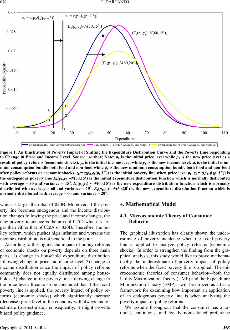 T. DARTANTO Copyright © 2011 SciRes. ME 670 Figure 1. An Illustration of Poverty Impact of Shifting the Expenditure Distribution Curve and the Poverty Line responding to Change in Price and Income Level. Source: Author; Note: p0 is the initial price level while p1 is the new price level as a result of policy reforms (economic shocks). y0 is the initial income level while y1 is the new income level. 0 is the initial mini- mum consumption bundle both food and non-food while 1 is the new minimum consumption bundle both food and non-food after policy reforms or economic shocks. z0 = z(p0, 0(p0,U*)) is the initial poverty line when price level p0. z1 = z(p1, 1(p1,U*)) is the endogenous poverty line. E0(p0,y0)N(50,152) is the initial expenditure distribution function which is normally distributed with average = 50 and variance = 152. E1(p1,y1) N(60,152) is the new expenditure distribution function which is normally distributed with average = 60 and variance = 152. E1(p1,y1) N(60,202) is the new expenditure distribution function which is normally distributed with average = 60 and variance = 202. 4. Mathematical Model which is larger than that of 020B. Moreover, if the pov- erty line becomes endogenous and the income distribu- tion changes following the price and income changes, the new poverty incidence is the area of 025D which is lar- ger than either that of 020A or 020B. Therefore, the po- licy reform, which pushes high inflation and worsens the income distribution, is not beneficial to the poor. 4.1. Microeconomic Theory of Consumer Behavior The graphical illustration has clearly shown the under- estimate of poverty incidence when the fixed poverty line is applied to analyze policy reforms (economic shocks). In order to strengthen the finding from the gra- phical analysis, this study would like to prove mathema- tically the underestimate of poverty impact of policy reforms when the fixed poverty line is applied. The mi- croeconomic theories of consumer behavior—both the Utility Maximization Theory (UMP) and the Expenditure Minimization Theory (EMP)—will be utilized as a basic framework for examining how important an application of an endogenous poverty line is when analyzing the poverty impact of policy reforms. According to this figure, the impact of policy reforms or economic shocks on poverty depends on three main parts: 1) change in household expenditure distribution following change in price and income level; 2) change in income distribution since the impact of policy reforms commonly does not equally distributed among house- holds; 3) change in the poverty line following change in the price level. It can also be concluded that if the fixed poverty line is applied, the poverty impact of policy re- forms (economic shocks) which significantly increase (decrease) price level in the economy will always under- estimate (overestimate); consequently, it might provide biased policy guidance. We assume throughout that the consumer has a ra- tional, continuous, and locally non-satiated preference  T. DARTANTO671 relation, and we take to be a continuous utility function representing this preference. The consumption set is in which l is a unit of commodity . The initial income is y which comes from selling its endowment of labor and capital for production activities. The price vector is Ux l R l 1i ,l il pp pR in which is the price of a unit of commodity . Therefore, the set of all feasible commodity bundles for the consumer is i p l 1i ,Bpyxpxy . The set is called the budget set of the con- sumer if his income is y and the price system is p. ,Bp y Then the optimization problem of a consumer with utility function , income y and price system p is subject to ,. This optimization results in the consumer’s demand function Ux maxUx px y0x , xpy. If , xp Vp y ,y is the consumer’s demand function, the indirect utility function of the consumer is which is given by Vp . The proper- ties of are strictly increasing in y for all p and non-increasing inifor all i=1,…,l (decreasing in p); homogeneous of degree zero in (p,y), continuous in (p,y), and quasi-convex in (p,y) [10]. 1l VR ,R y py ,Ux p On the other hand, the consumer can also look for a commodity bundle which guarantees him to achieve a utility level with minimum expenditure y. This is well known as the expenditure minimization problem (EMP). The value of the EMP is denoted Ux ,epU which is called the consumer’s expenditure function. Its value for any is simply , where ,pU px is any solution to the EMP. The properties of are strictly increasing in for every p and non-decreasing in i for all i = 1,…,i; homogeneous of degree one in p; concave in p; continuous in p and U [10]. The set of opti- mal commodity in the EMP is denoted and is known as the Hicksian, or compensated, demand corre- spondence or function if single-valued. One of the pro- perties of the Hicksian demand corresp o nde nce ,U U ep , U p hp ,hp hp U U is homogeneity of degree zero in p: for any p, U and hp ,,U0 [10]. If the is the solution to the Utility Maximization Problem (UMP) when , in which 0ypx is a solution to the problem of maximization subject to and , then Ux px y0x Ux is also the solution of the Expenditure Minimization Problem (EMP) when the required utility level is . Moreover, the mini- mized expenditure level in this EMP is exactly y. If the is optimal in the EMP when required utility level is , then Ux 0U is optimal in the UMP when income is px . Moreover, the maximized utility level in this UMP is exactly U. The EMP is the “dual” problem to the UMP. From UMP and EMP, then we have: e,e,e, ,ypxpUpUxpVpy [10] ,, ,e,UUx VpyVppxVppU [11] ,,,e,hpUx pyx ppU [12] ,,, pyhpV py [13] 4.2. Poverty Function Even though, there are many definitions, measurements and characteristics of poverty, this study simplify defines that poverty is those with consumption expenditure be- low the line a re cons idered “p oor’’ and the rest ar e “non- poor’’. According to [11-16], it could be summarized that the poverty (HC) is a function of the welfare indica- tor (w), the poverty line (z) and the income distribution . The poverty function is shown as follows: ,,HCfw z [14] The properties of poverty function are continuous and decreasing in w, continuous and increasing in both z and . Decreasing in w implies poverty indicators will de- crease following an increase in the welfare indicators. The measurable welfare indicators commonly used in analyzing poverty are either income or expenditure. Meanwhile, increases in both z and implies that poverty indicators will increase in line with an increase in the poverty line and the income distribution. Su- pposing the expenditure as the welfare indicator and fol- lowing Equation 10, then we have the welfare function shown be low: e,e, ,wypxpUpVp y [15] On the other hand, the ideal poverty line should then be the minimum cost to a given individual of a reference level of welfare fixed across all individuals, * U [1]. Thus, the poverty line can be defined as cost of achieving * U when facing price vector p and the vector of consumption bundle . The vector of consumption bundle is a function of p and , ,the Hicksian demand correspondence. is the mi- nimum consumption bundle to achieve (e.g. 2,100 calories) when price vector is p. According to Equation 12 and Equation 13, * U * ,pU * pU* U , * ,pU must be equal to ,py , the demand function. Thus, the poverty line can be shown as below: * ,,zzppU [16] The poverty line, * ,,zzppU , is continuously increasing in p and . Suppose is a fixed value overtime1, then * U ** 0 ttUU , and the one property 1The utility is fixed because the standard reference of welfare as abasis of calculation of poverty line is not easily changed overtime. For in- stance, the minimum standard of 2,100 calories for measuring the pov- erty line does not change for many years. Copyright © 2011 SciRes. ME  T. DARTANTO 672 of the Hicksian demand correspondence is the homoge- neity of degree zero in p, then *0U and 0p . Lastly, let us simplify that the income distribution, which is mainly measured by either the Gini Index or Theil Index, is a function of the distribution of endow- ments among households in a society. Endow- ments could be defined as labor, capital, land ownership and education attainment etc. Let us assume that the properties of income distribution are continuous and in- creasing in . Increasing in means an unequal dis- tribution of endowments in society related to more un- equal in income distribution. The income distribution function is shown below: [17] Substituting Equation 17, Equation 16, Equation 15 into Equation 14, then we obtain the poverty function as shown be low: * e,,,,,,HCfpVpyzpp U [18] 4.3. The Mathematical Proof of Different Poverty Outcome As mentioned in the graphical analysis, if the fixed po- verty line is applied, the poverty impact of policy re- forms (economic shocks) which increase the price level will always be underestimated. This study will mathe- matically prove the evidence from the graphical analysis by utilizing Equation 18 and the properties of expendi- ture function, indirect utility function, poverty function and income distribution function. Proposition: Supposing the application of a fixed poverty line, the poverty impact of policy reforms which largely increase (decrease) the price level, will always be underestimated (overestimated). Proof: Let us take the total derivate of Equation 18 and if dd;; ; tept ; CHCtffeeepppt ; V eeV ; p VVp ; y VVy ; t yy t ; z fz ; p zzp ;zz ; pp **; U zzU **; UU ** ; t UU t ;ff ; and tt then we have: ** * tepteVpt eVy zptzpt zt t UU t Cfep feVp feVy fzp fzp fzU f [19a] Suppose (there is no change in the reference of utility, ) and *0 t U * U0 p (the homogeneity of degree zero in p), then Equation 19(a) will be: tepteVpt eVyt zpt t CfepfeVpfeVy fzpf [19b] Suppose 0; e f 0; p e 0; t p 0; V e0; p V 0; y V 0; t y 0; z f 0; p z 0;f 0; 0; t If ep teVyt eVpz pt fe pfeVy feV pfzpf , then the sign of change in poverty (HC) is negative. It means that the policy reforms or economic shocks bene- fit the poor. On the contrary, if ep teVyt eVpz pt fe pfeVy feV pfz pf , then the sign of change in poverty (HC) is positive meaning the policy reforms or economic shocks do not benefit the poor. Equation 19(b) intuitively shows that the change in poverty responding to policy reforms or economic shocks depends on five components: 1) change in house- hold expenditure as a result of a change in price, 2) change in household expenditure as a response to utility change due to a change in price, 3) change in household expenditure as a response to utility change due to a change in income, 4) change in poverty line as a response to a price change, 5) change in income distribution as a re- sponse to a change in endowment. Equation 19(b) rep resents the pov erty impact of po licy reforms under the endogenous poverty line. The part of pt zp in Equation 19(b) is the change of the pov- erty indicator contributed by the change in the poverty line. Deleting pt zp in Equation 19(b), then we have: fix tepteVp eVy tt CfepfeVp feVy f [20] Equation 20 represents the poverty impact of policy reforms under the fixed poverty line. There is no change in the poverty indicator contributed by the change in the poverty line. The different poverty outcome between applying the endogenous poverty line and the fixed pov- erty line can be calculated by deducting Equation 20 from Equation 19(b). The different outcome is shown below: 0 fix tt zpt HCHCf zp [21] According to Equation 21, if , the poverty outcome under the endogenous poverty line will always be large than that of the fixed poverty line. However, if the policy reforms or economic shocks did not affect the 0 t p Copyright © 2011 SciRes. ME  T. DARTANTO Copyright © 2011 SciRes. ME 673 price level, then the poverty outcome either under the endogenous poverty line or the fixed poverty line will be equal. Therefore, the proposition, that if the fixed pover- ty line is applied, the poverty impact of policy reforms which largely increase (decrease) the price level will always be underestimated (overestimated) can be math- ematically proven. QED 5. Concluding Remarks Policy reforms (economic shocks) that increase the price level will have a double effect on poverty: 1) reduce the purchasing power and 2) increase the poverty line. Most of studies on the poverty impact of policy reforms do not pay much attention to the second effect, as the poverty line is assumed as a fixed line; thus, the poverty outcome of pol- icy reforms may underestimate (overestimate) and mislead in policy guidance. The graphical analysis and the mathe- matical model have clearly showed how important an ap- plication of an endogenous poverty line is when analyzing the poverty impact of policy reforms. Applying the microeconomic theory of consumer be- havior and the properties of poverty function, this study has theoretically proven that, under the fixed poverty line, the poverty impact of policy reforms (economic shocks) which significantly increase (decrease) price will always be un- derestimated (overestimated). However, if the policy re- forms (economics shocks) do not change the price level in the economy, applying either the fixed poverty line or the endogenous poverty line will result in a similar outcome. Since this is difficult to guarantee that the policy reforms do not change the price level, thus, this study suggests that the endogenous poverty line should be applied when ana- lyzing the poverty impacts of policy reforms. Moreover, the empirical investigation should be done in order to strengthen the finding from the graphical analysis and the mathem atical m odel. 6. Acknowledgements The author would like to thank the participants at the Monthly Discussion at the Department of Economics, University of Indonesia, on September 30, 2010, and Prof. Shigeru Otsubo for their valuable comments. Any remaining errors are the author’s responsibility. 7. References [1] M. Ravallion, “Poverty Comparisons. Fundamentals of Pure and Applied Economic,” Vol. 56, Harwood Aca- demic Press, Chur, Switzerland, 1994. [2] L. B. Decaluwé, L. Savard and E. Thorbecke, “General Equilibrium Approach for Poverty Analysis: with an Ap- plication to Cameroon,” African Development Review, Vol. 17, No. 2, 2005, pp. 213-243. doi:10.1111/j.1017-6772.2005.00113.x [3] Azis and J. Iwan, “Macro Stability Can Be Detrimental to Poverty,” Economics and Finance Indonesia, Vol. 57, No. 1, 2010, pp. 1-23. [4] Powers and T. Elizabeth, “Inflation, Unemployment and Poverty Revisited,” Economic Review, Federal Reserve Bank of Cleveland, Quarter 3, 1995, pp. 2-13. [5] Datt, Gaurav, and M. Ravallion, “Why Have Some Indian States Done Better Than Others at Reducing Rural Pov- erty?” World Bank Policy Research Work ing Paper 1594, April 1996. [6] Agenor and Pierre-Richard, “Stabilization Policies,” Pov- erty and the Labor Market Mimeo Paper, IMF and World Bank, 1998. [7] Son, H. Hyun and N. Kakwani, “Measuring the Impact of Price Changes on Poverty,” International Poverty Center, UNDP, Working Paper Number 33, November 2006, ac- cessed at 7 July 2010. http://www.ipc-undp.org/pub/IPCWorkingPaper33.pdf [8] M. Ravallion, “Poverty Line in Theory and Practice,” The World Bank: LSMS Working Paper Number 133, 1998. [9] A. Hagenaars and V. de Klaas, “The Definition and Measurement of Poverty,” Journal of Human Resources, Vol. 23, No.2, 1988, pp. 211-221. [10] A. Mas-Collel, M. D. Whinston and J. R. Green, “Micro- economic Theory,” Oxford University Press, New York, 1995. [11] Atkinson and B. Anthony, “On the Measurement of Ine- quality,” Journal of Public Theory, Vol. 2, 1970, pp. 244- 263. [12] J. E. Foster, J. Greer and E. Thorbecke, “A Class of De- composable Poverty Measures,” Econometrica, Vol. 52, 1984, pp. 761-776. [13] N. Kakwani, “On a Class of Poverty Measures,” Econometrica, Vol. 48, No. 2, 1980, pp. 437-446. [14] N. Kakwani, “Poverty and Economic Growth with Ap- plication to Cote D’Ivore,” Review of Income and Wealth, Series 39, Number 2, June 1993. [15] A. Sen, “An Ordinal Approach to Measurement,” Econometrica, Vol. 44, No. 2, March 1976, pp. 219-231. [16] A. Sen, “On Economic Inequality,” Clarendon Press, Oxford, 1973.
|