Modern Economy, 2011, 2, 633-641
doi:10.4236/me.2011.24071 Published Online September 2011 (http://www.SciRP.org/journal/me)
Environmental Policy and Pollution Dynamics in an
Economic Growth Model
Weibin Zhang
Ritsumeikan Asia Pacific University, Beppu -shi, Japan
Received April 26, 2011; revised May 29, 2011; accept ed June 13, 2011
Abstract
The purpose of this paper is to study dynamic interactions among capital accumulation, environmental
change and labor distribution. We try to synthesize the growth mechanism in the neoclassical growth theory
and the environmental dynamics in traditional models of environmental economics within a comprehensive
framework with an alternative approach to household behavior. We build a model which describes a dy-
namic interdependence among physical accumulation, environmental change and division of labor under
perfect competition with environmental taxes on production, wealth income, wage income and consumption.
We simulate the model to demonstrate existence of equilibrium points and motion of the dynamic system.
The simulation demonstrates some dynamics which can be predicted neither by the neoclassical growth the-
ory Solow model nor by the traditional economic models of environmental change.
Keywords: The Environmental Kuznets Curve, Environmental Tax, Economic Growth, Capital
Accumulation, Labor Distribution
1. Introduction
The purpose of this study is to study interactions between
environmental change and economic growth. In recent
years environmental issues have received more attention
than ever. Global warming threatens living conditions of
mankind and local environmental catastrophes are daily
reported in TVs. It is challenging for economists to ex-
plain economic mechanisms and consequences of envi-
ronmental changes. Environmental issues have increas-
ingly caused attention in the literature of economic
growth and development (see [1-3]). As mentioned by
[4], one can find three effects that are important in ex-
plaining the level of environmental pollution and re-
source use. The three effects are: 1) increases in output
tends to require more inputs and produce more emissions;
2) changes in income or preferences may lead to policy
changes which will affect production and thus emission;
and 3) as income increases, the economic structure may
be changed which will causes changes in the environ-
ment (see [5-7]). It is argued that the net effect of these
effects tends to result in the environmental Kuznets
curve. Kuznets [8] postulated that economic growth and
income inequalities follow an inverted U-curve. The en-
vironmental Kuznets curve refers to the same relation
between environmental quality and per capita income. A
recent survey on the economic models for the curve is
given by [7]. Nevertheless, a large number of empirical
studies on the environmental Kuznets curve for various
pollutants find different relations—for instance, inverted
U-shaped relationship, a U-shaped relationship, a mono-
tonically increasing or monotonically decreasing rela-
tionship—between pollution and rising per capita income
levels (see [4,9,10]). The ambiguous or situation-de-
pendent relations between environmental quality and
economic growth and the inability of economic growth
theory for properly explaining these observed phenom-
ena implies the necessity that more comprehensive theo-
ries are needed.
Economic growth often implies worsened environ-
mental conditions. Growth also implies a higher material
standard of living which will, through the demand for a
better environment induces changes in the structure of
the economy to improve environment. As a society ac-
cumulates more capital and makes progresses in tech-
nology, more resources may be used to protect environ-
ment. Tradeoffs between consumption and pollution
have been extensively analyzed since the publication of
the seminal papers by [11,12]. Issues related to interde-
pendence between economic growth and environment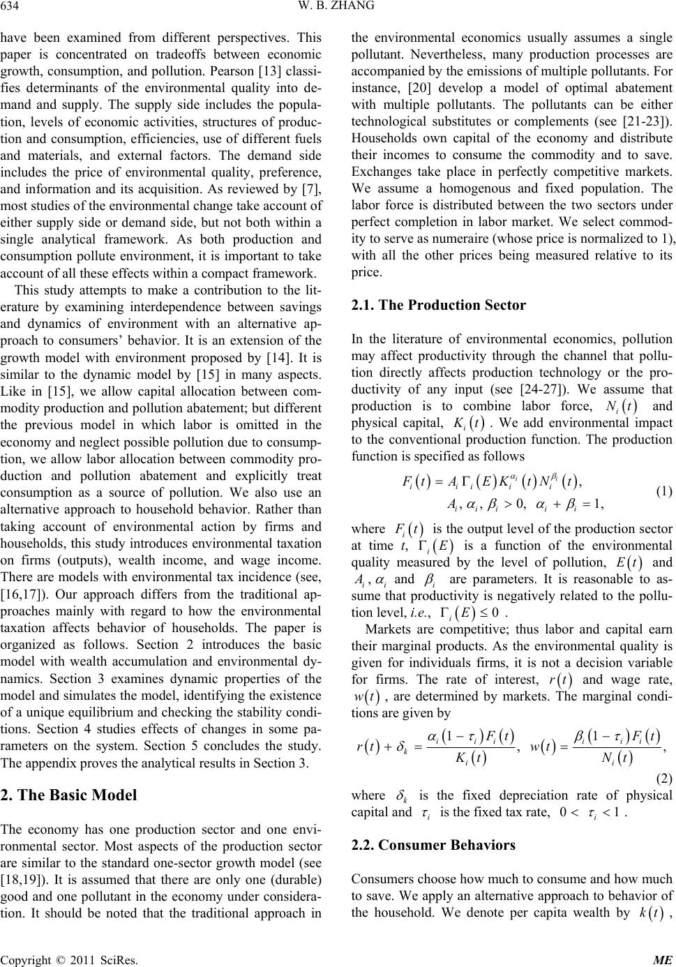

W. B. ZHANG 634
have been examined from different perspectives. This
paper is concentrated on tradeoffs between economic
growth, consumption, and pollution. Pearson [13] classi-
fies determinants of the environmental quality into de-
mand and supply. The supply side includes the popula-
tion, levels of economic activities, structures of produc-
tion and consumption, efficiencies, use of different fuels
and materials, and external factors. The demand side
includes the price of environmental quality, preference,
and information and its acquisition. As reviewed by [7],
most studies of the environmental change take account of
either supply side or demand side, but not both within a
single analytical framework. As both production and
consumption pollute environment, it is important to take
account of all these effects within a compact framework.
This study attempts to make a contribution to the lit-
erature by examining interdependence between savings
and dynamics of environment with an alternative ap-
proach to consumers’ behavior. It is an extension of the
growth model with environment proposed by [14]. It is
similar to the dynamic model by [15] in many aspects.
Like in [15], we allow capital allocation between com-
modity production and pollution abatement; but different
the previous model in which labor is omitted in the
economy and neglect possible pollution due to consump-
tion, we allow labor allocation between commodity pro-
duction and pollution abatement and explicitly treat
consumption as a source of pollution. We also use an
alternative approach to household behavior. Rather than
taking account of environmental action by firms and
households, this study introduces environmental taxation
on firms (outputs), wealth income, and wage income.
There are models with environmental tax incidence (see,
[16,17]). Our approach differs from the traditional ap-
proaches mainly with regard to how the environmental
taxation affects behavior of households. The paper is
organized as follows. Section 2 introduces the basic
model with wealth accumulation and environmental dy-
namics. Section 3 examines dynamic properties of the
model and simulates the model, identifying the existence
of a unique equilibrium and checking the stability condi-
tions. Section 4 studies effects of changes in some pa-
rameters on the system. Section 5 concludes the study.
The appendix proves the analytical results in Section 3.
2. The Basic Model
The economy has one production sector and one envi-
ronmental sector. Most aspects of the production sector
are similar to the standard one-sector growth model (see
[18,19]). It is assumed that there are only one (durable)
good and one pollutant in the economy under considera-
tion. It should be noted that the traditional approach in
the environmental economics usually assumes a single
pollutant. Nevertheless, many production processes are
accompanied by the emissions of multiple pollutants. For
instance, [20] develop a model of optimal abatement
with multiple pollutants. The pollutants can be either
technological substitutes or complements (see [21-23]).
Households own capital of the economy and distribute
their incomes to consume the commodity and to save.
Exchanges take place in perfectly competitive markets.
We assume a homogenous and fixed population. The
labor force is distributed between the two sectors under
perfect completion in labor market. We select commod-
ity to serve as numeraire (whose price is normalized to 1),
with all the other prices being measured relative to its
price.
2.1. The Production Sector
In the literature of environmental economics, pollution
may affect productivity through the channel that pollu-
tion directly affects production technology or the pro-
ductivity of any input (see [24-27]). We assume that
production is to combine labor force,


i
Nt and
physical capital,


i
K
t. We add environmental impact
to the conventional production function. The production
function is specified as follows




,
,, 0,1,
ii
iiiii
iiii i
Ft AEKtNt
A

 


(1)
where


i
F
t is the output level of the production sector
at time t,


E
i
 is a function of the environmental
quality measured by the level of pollution,


Et and
,
i
Ai

and i

are parameters. It is reasonable to as-
sume that productivity is negatively related to the pollu-
tion level, i.e.,


0E
i

.
Markets are competitive; thus labor and capital earn
their marginal products. As the environmental quality is
given for individuals firms, it is not a decision variable
for firms. The rate of interest, and wage rate,

rt


wt , are determined by markets. The marginal condi-
tions are given by





 




11
,,
iii iii
kii
F
tF
rt wt
Kt Nt
 


 t
(2)
where k

is the fixed depreciation rate of physical
capital and i

is the fixed tax rate, 01
i

.
2.2. Consumer Behaviors
Consumers choose how much to consume and how much
to save. We apply an alternative approach to behavior of
the household. We denote per capita wealth by


kt ,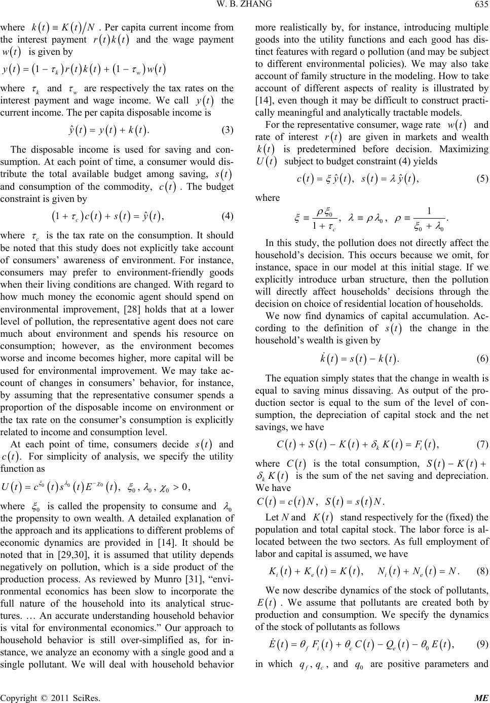

W. B. ZHANG635
where
 
ktKt N. Per capita current income from
the interest payment and the wage payment
is given by
 
rtkt
 
11

wt
    
kw
y
tr tkt   wt
where k

and w

are respectively the tax rates on the
interest payment and wage income. We call


y
t the
current income. The per capita disposable income is
 
ˆ.

y
tytkt (3)
The disposable income is used for saving and con-
sumption. At each point of time, a consumer would dis-
tribute the total available budget among saving,


s
t
and consumption of the commodity, . The budget
constraint is given by

ct
 
ˆ
1,
cyt
 
 
ct st (4)
where c

is the tax rate on the consumption. It should
be noted that this study does not explicitly take account
of consumers’ awareness of environment. For instance,
consumers may prefer to environment-friendly goods
when their living conditions are changed. With regard to
how much money the economic agent should spend on
environmental improvement, [28] holds that at a lower
level of pollution, the representative agent does not care
much about environment and spends his resource on
consumption; however, as the environment becomes
worse and income becomes higher, more capital will be
used for environmental improvement. We may take ac-
count of changes in consumers’ behavior, for instance,
by assuming that the representative consumer spends a
proportion of the disposable income on environment or
the tax rate on the consumer’s consumption is explicitly
related to income and consumption level.
At each point of time, consumers decide


s
t and
For simplicity of analysis, we specify the utility
function as

.ct

Ut
 
00
00 0
,,,0c ts t

 

0
E t
 ,
where 0

is called the propensity to consume and 0

the propensity to own wealth. A detailed explanation of
the approach and its applications to different problems of
economic dynamics are provided in [14]. It should be
noted that in [29,30], it is assumed that utility depends
negatively on pollution, which is a side product of the
production process. As reviewed by Munro [31], “envi-
ronmental economics has been slow to incorporate the
full nature of the household into its analytical struc-
tures. … An accurate understanding household behavior
is vital for environmental economics.” Our approach to
household behavior is still over-simplified as, for in-
stance, we analyze an economy with a single good and a
single pollutant. We will deal with household behavior
more realistically by, for instance, introducing multiple
goods into the utility functions and each good has dis-
tinct features with regard o pollution (and may be subject
to different environmental policies). We may also take
account of family structure in the modeling. How to take
account of different aspects of reality is illustrated by
[14], even though it may be difficult to construct practi-
cally meaningful and analytically tractable models.
For the representative consumer, wage rate


wt and
rate of interest


rt are given in markets and wealth


kt is predetermined before decision. Maximizing


Ut subject to budget constraint (4) yields






ˆ
,ctyt styt  

ˆ
,  (5)
where
0
0
00
1
,,
1c


.




In this study, the pollution does not directly affect the
household’s decision. This occurs because we omit, for
instance, space in our model at this initial stage. If we
explicitly introduce urban structure, then the pollution
will directly affect households’ decisions through the
decision on choice of residential location of households.
We now find dynamics of capital accumulation. Ac-
cording to the definition of 

s
t the change in the
household’s wealth is given by




.kt stkt


(6)
The equation simply states that the change in wealth is
equal to saving minus dissaving. As output of the pro-
duction sector is equal to the sum of the level of con-
sumption, the depreciation of capital stock and the net
savings, we have






,
ki
Ct St KtKt Ft   

(7)
where


Ct is the total consumption,



St Kt




k
K
t 
is the sum of the net saving and depreciation.
We have








,.CtctN StstN
Let N and


K
t stand respectively for the (fixed) the
population and total capital stock. The labor force is al-
located between the two sectors. As full employment of
labor and capital is assumed, we have






,
ie
K
tKtKt (8)
 
.
ie
Nt NtN
We now describe dynamics of the stock of pollutants,


Et . We assume that pollutants are created both by
production and consumption. We specify the dynamics
of the stock of pollutants as follows





 
0, fi ce
EtFtCtQ tEt   


(9)
in which ,
f
c
qq, and are positive parameters and
0
q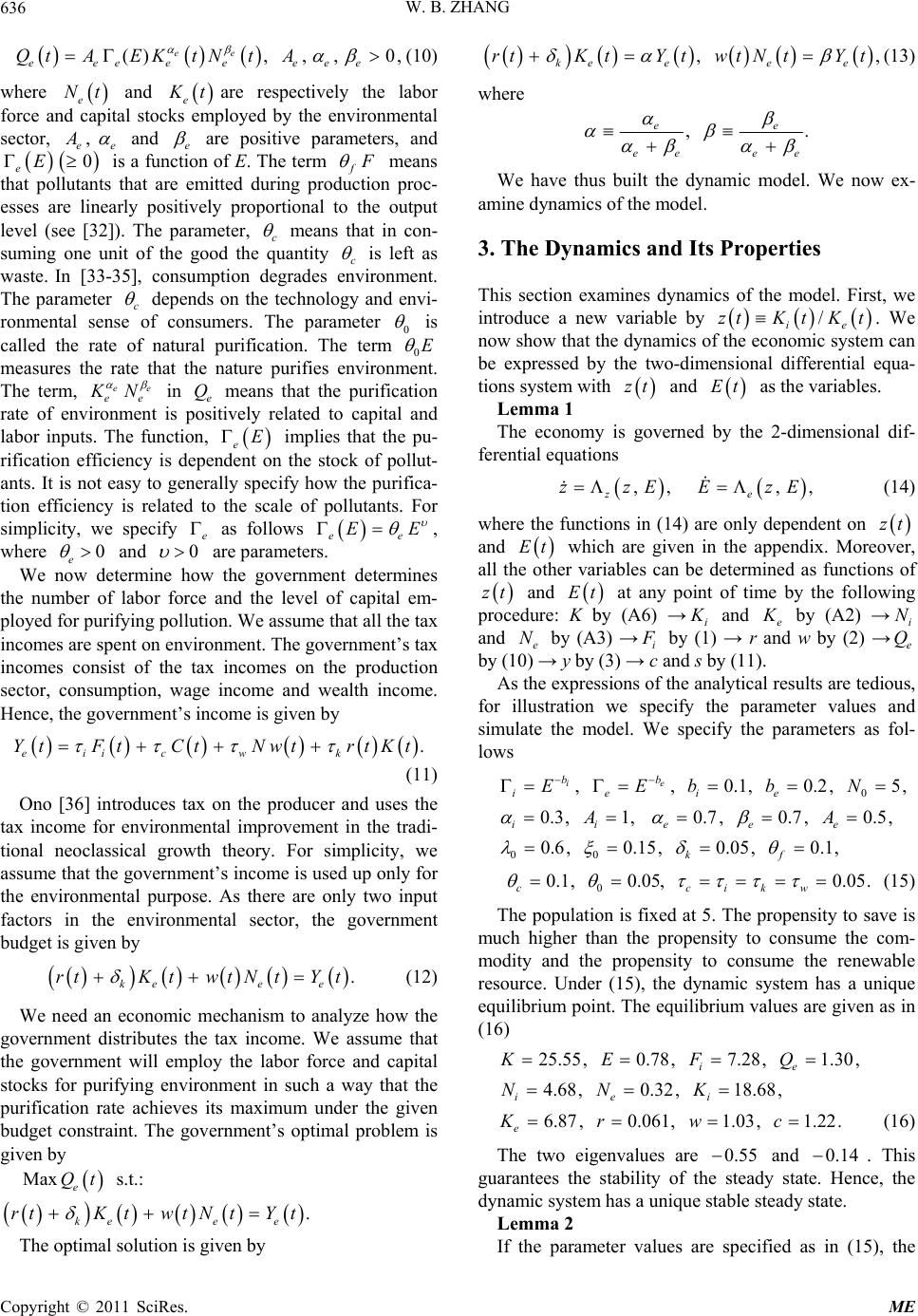

W. B. ZHANG 636
 


(),, ,0,
ee
eeeeeeee
Qt AEKtNtA

  (10)
where and

e
Nt

e
K
tare respectively the labor
force and capital stocks employed by the environmental
sector, ,
e
A
e

and e

are positive parameters, and
e is a function of E. The term f

E
 
0
F

means
that pollutants that are emitted during production proc-
esses are linearly positively proportional to the output
level (see [32]). The parameter, c

means that in con-
suming one unit of the good the quantity c

is left as
waste. In [33-35], consumption degrades environment.
The parameter c

depends on the technology and envi-
ronmental sense of consumers. The parameter 0

is
called the rate of natural purification. The term 0E

measures the rate that the nature purifies environment.
The term, ee
ee
K
N


in e Q means that the purification
rate of environment is positively related to capital and
labor inputs. The function, e implies that the pu-
rification efficiency is dependent on the stock of pollut-
ants. It is not easy to generally specify how the purifica-
tion efficiency is related to the scale of pollutants. For
simplicity, we specify e as follows ee

E


EE

  ,
where 0
e

 and 0

 are parameters.
We now determine how the government determines
the number of labor force and the level of capital em-
ployed for purifying pollution. We assume that all the tax
incomes are spent on environment. The government’s tax
incomes consist of the tax incomes on the production
sector, consumption, wage income and wealth income.
Hence, the government’s income is given by
 


.
eiic wk
Yt FtCtNwtrtKt   
(11)
Ono [36] introduces tax on the producer and uses the
tax income for environmental improvement in the tradi-
tional neoclassical growth theory. For simplicity, we
assume that the government’s income is used up only for
the environmental purpose. As there are only two input
factors in the environmental sector, the government
budget is given by
   
.
kee e
rtKtwtNtYt    (12)
We need an economic mechanism to analyze how the
government distributes the tax income. We assume that
the government will employ the labor force and capital
stocks for purifying environment in such a way that the
purification rate achieves its maximum under the given
budget constraint. The government’s optimal problem is
given by

Max e Qt
 
ke
rt K 
s.t.:

.
e e
twtNtYt 
The optimal solution is given by










,,
ke eee
rtKtYt wtNtYt    (13)
where
,.
ee
ee ee







We have thus built the dynamic model. We now ex-
amine dynamics of the model.
3. The Dynamics and Its Properties
This section examines dynamics of the model. First, we
introduce a new variable by
 


/
ie
ztK tKt. We
now show that the dynamics of the economic system can
be expressed by the two-dimensional differential equa-
tions system with


zt and as the variables.

Et
Lemma 1
The economy is governed by the 2-dimensional dif-
ferential equations


,
z
zzE
, , (14)

,
e
EzE

where the functions in (14) are only dependent on


zt
and


Et which are given in the appendix. Moreover,
all the other variables can be determined as functions of


zt and


Et at any point of time by the following
procedure: K by (A6) →i
K
and e
K
by (A2) →
and e by (A3) →i
i
N
N
F
by (1) → r and w by (2) →
by (10) → y by (3) → c and s by (11).
e
Q
As the expressions of the analytical results are tedious,
for illustration we specify the parameter values and
simulate the model. We specify the parameters as fol-
lows
0
,, 0.1,0.2,5,
ie
bb
ieie
EEbbN


 
0.3, 1,0.7,0.7,0.5,
iieee
AA




 
00
0.6,0.15,0.05,0.1,
kf




0
0.1, 0.05,0.05.
ccikw



 (15)
The population is fixed at 5. The propensity to save is
much higher than the propensity to consume the com-
modity and the propensity to consume the renewable
resource. Under (15), the dynamic system has a unique
equilibrium point. The equilibrium values are given as in
(16)
25.55, 0.78,7.28,1.30,
ie
KEFQ

 
4.68,0.32, 18.68,
iei
NNK


6.87,0.061,1.03, 1.22.
e
Krwc

 (16)
The two eigenvalues are and . This
guarantees the stability of the steady state. Hence, the
dynamic system has a unique stable steady state.
0.550.14
Lemma 2
If the parameter values are specified as in (15), the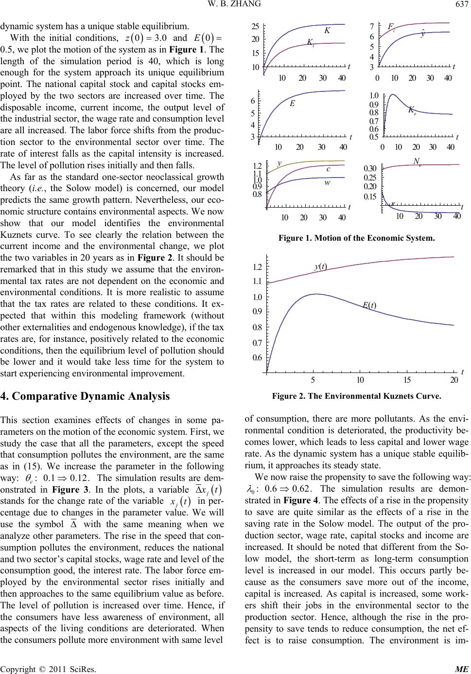

W. B. ZHANG637
0
dynamic system has a unique stable equilibrium.
With the initial conditions, and

03.z


0E

0.5, we plot the motion of the system as in Figure 1. The
length of the simulation period is 40, which is long
enough for the system approach its unique equilibrium
point. The national capital stock and capital stocks em-
ployed by the two sectors are increased over time. The
disposable income, current income, the output level of
the industrial sector, the wage rate and consumption level
are all increased. The labor force shifts from the produc-
tion sector to the environmental sector over time. The
rate of interest falls as the capital intensity is increased.
The level of pollution rises initially and then falls.
As far as the standard one-sector neoclassical growth
theory (i.e., the Solow model) is concerned, our model
predicts the same growth pattern. Nevertheless, our eco-
nomic structure contains environmental aspects. We now
show that our model identifies the environmental
Kuznets curve. To see clearly the relation between the
current income and the environmental change, we plot
the two variables in 20 years as in Figure 2. It should be
remarked that in this study we assume that the environ-
mental tax rates are not dependent on the economic and
environmental conditions. It is more realistic to assume
that the tax rates are related to these conditions. It ex-
pected that within this modeling framework (without
other externalities and endogenous knowledge), if the tax
rates are, for instance, positively related to the economic
conditions, then the equilibrium level of pollution should
be lower and it would take less time for the system to
start experiencing environmental improvement.
4. Comparative Dynamic Analysis
This section examines effects of changes in some pa-
rameters on the motion of the economic system. First, we
study the case that all the parameters, except the speed
that consumption pollutes the environment, are the same
as in (15). We increase the parameter in the following
way: :0.1 0.12.
c

 The simulation results are dem-
onstrated in Figure 3. In the plots, a variable


j
x
t
stands for the change rate of the variable


j
x
t in per-
centage due to changes in the parameter value. We will
use the symbol  with the same meaning when we
analyze other parameters. The rise in the speed that con-
sumption pollutes the environment, reduces the national
and two sector’s capital stocks, wage rate and level of the
consumption good, the interest rate. The labor force em-
ployed by the environmental sector rises initially and
then approaches to the same equilibrium value as before.
The level of pollution is increased over time. Hence, if
the consumers have less awareness of environment, all
aspects of the living conditions are deteriorated. When
the consumers pollute more environment with same level
102030 40
10
15
20
25
010 2030 40
3
4
5
6
7
10 20 30 40
3
4
5
6
01020 3040
0.5
0.6
0.7
0.8
0.9
1.0
10 20 30 40
0.8
0.9
1.0
1.1
1.2
10 20 30 40
0.15
0.20
0.25
0.30
K
K
i
t t
t
tt
t
F
i
K
e
N
e
E
c
w
r
y
ˆ
y
Figure 1. Motion of the Economic System.
510 15 20
0.6
0.7
0.8
0.9
1.0
1.1
1.2
y (t)
E(t)
t
Figure 2. The Environmental Kuznets Curve.
of consumption, there are more pollutants. As the envi-
ronmental condition is deteriorated, the productivity be-
comes lower, which leads to less capital and lower wage
rate. As the dynamic system has a unique stable equilib-
rium, it approaches its steady state.
We now raise the propensity to save the following way:
0: 0.60.62.

 The simulation results are demon-
strated in Figure 4. The effects of a rise in the propensity
to save are quite similar as the effects of a rise in the
saving rate in the Solow model. The output of the pro-
duction sector, wage rate, capital stocks and income are
increased. It should be noted that different from the So-
low model, the short-term as long-term consumption
level is increased in our model. This occurs partly be-
cause as the consumers save more out of the income,
capital is increased. As capital is increased, some work-
ers shift their jobs in the environmental sector to the
production sector. Hence, although the rise in the pro-
pensity to save tends to reduce consumption, the net ef-
fect is to raise consumption. The environment is im-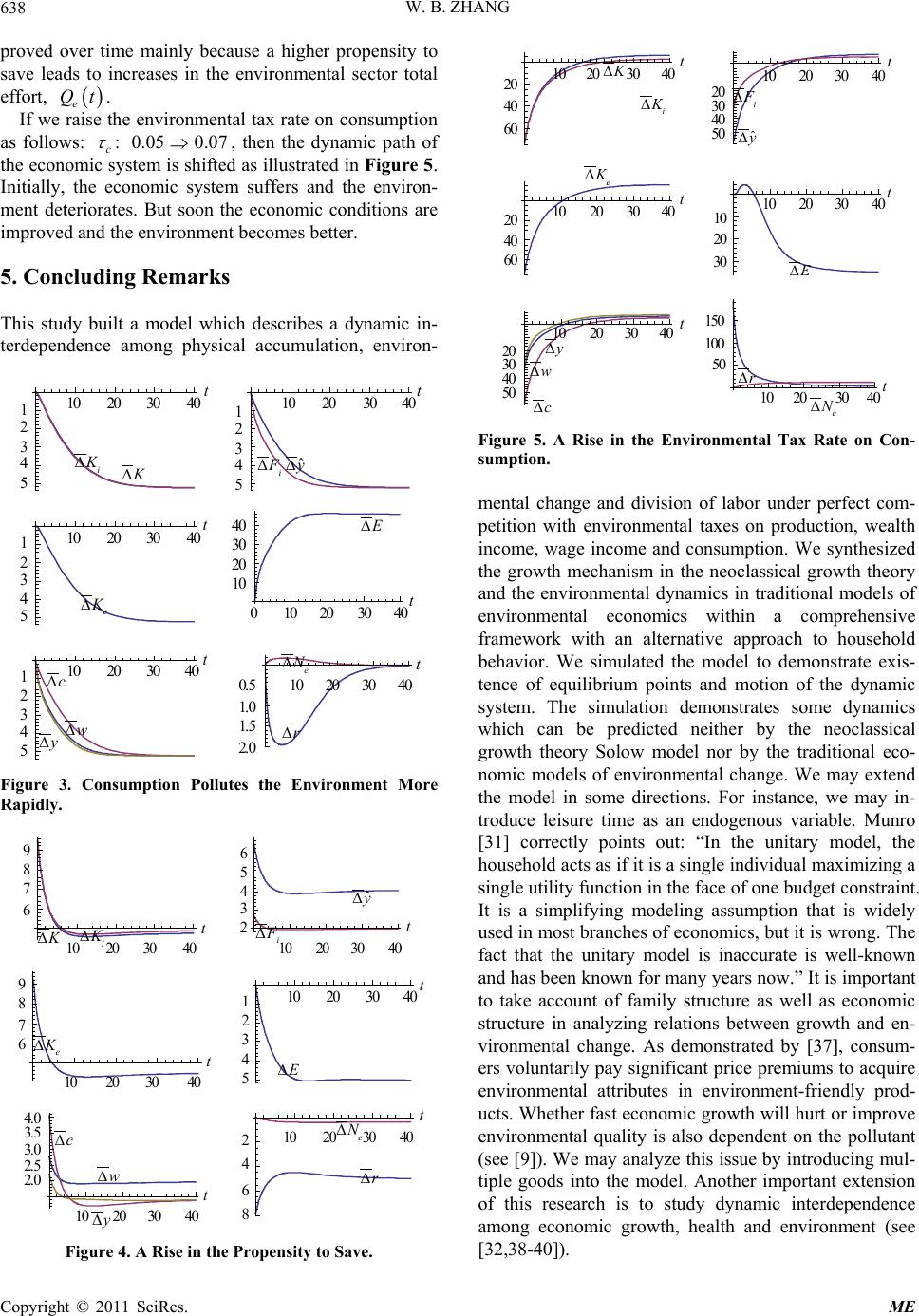

W. B. ZHANG 638
proved over time mainly because a higher propensity to
save leads to increases in the environmental sector total
effort, .

e
Qt
c
If we raise the environmental tax rate on consumption
as follows: :0.05 0.07

, then the dynamic path of
the economic system is shifted as illustrated in Figure 5.
Initially, the economic system suffers and the environ-
ment deteriorates. But soon the economic conditions are
improved and the environment becomes better.
5. Concluding Remarks
This study built a model which describes a dynamic in-
terdependence among physical accumulation, environ-
10 2030 40
5
4
3
2
1102030 40
5
4
3
2
1
10 2030 40
5
4
3
2
1
010 203040
10
20
30
40
102030 40
5
4
3
2
110 20 30 40
2. 0
1. 5
1. 0
0. 5
t
t
t
K∆
K
i
∆
tt
t
F
i
∆
K
e
∆
N
e
∆
E∆
c∆
w∆
r∆
y
ˆ
∆
y∆
Figure 3. Consumption Pollutes the Environment More
Rapidly.
10 20 3040
6
7
8
9
10 20 30 40
2
3
4
5
6
10 2030 40
6
7
8
910 20 30 40
5
4
3
2
1
10203040
2. 0
2. 5
3. 0
3. 5
4. 0
10 20 30 40
8
6
4
2
K∆
K
i
∆
F
i
∆
K
e
∆
E∆
c∆
r∆
y
ˆ
∆
y∆
t
t
t
w∆
t
t
t
N
e
∆
Figure 4. A Rise in the Propensity to Save.
10 2030 40
60
40
20 10 20 30 40
50
40
30
20
1020 30 40
60
40
20
10 20 30 40
30
20
10
1020 30 40
50
40
30
20
10 2030 40
50
100
150
K∆
K
i
∆
t
t
t
t
t
t
F
i
∆
K
e
∆
N
e
∆
E∆
c∆
w∆r∆
y
ˆ
∆
y∆
Figure 5. A Rise in the Environmental Tax Rate on Con-
sumption.
mental change and division of labor under perfect com-
petition with environmental taxes on production, wealth
income, wage income and consumption. We synthesized
the growth mechanism in the neoclassical growth theory
and the environmental dynamics in traditional models of
environmental economics within a comprehensive
framework with an alternative approach to household
behavior. We simulated the model to demonstrate exis-
tence of equilibrium points and motion of the dynamic
system. The simulation demonstrates some dynamics
which can be predicted neither by the neoclassical
growth theory Solow model nor by the traditional eco-
nomic models of environmental change. We may extend
the model in some directions. For instance, we may in-
troduce leisure time as an endogenous variable. Munro
[31] correctly points out: “In the unitary model, the
household acts as if it is a single individual maximizing a
single utility function in the face of one budget constraint.
It is a simplifying modeling assumption that is widely
used in most branches of economics, but it is wrong. The
fact that the unitary model is inaccurate is well-known
and has been known for many years now.” It is important
to take account of family structure as well as economic
structure in analyzing relations between growth and en-
vironmental change. As demonstrated by [37], consum-
ers voluntarily pay significant price premiums to acquire
environmental attributes in environment-friendly prod-
ucts. Whether fast economic growth will hurt or improve
environmental quality is also dependent on the pollutant
(see [9]). We may analyze this issue by introducing mul-
tiple goods into the model. Another important extension
of this research is to study dynamic interdependence
among economic growth, health and environment (see
[32,38-40]).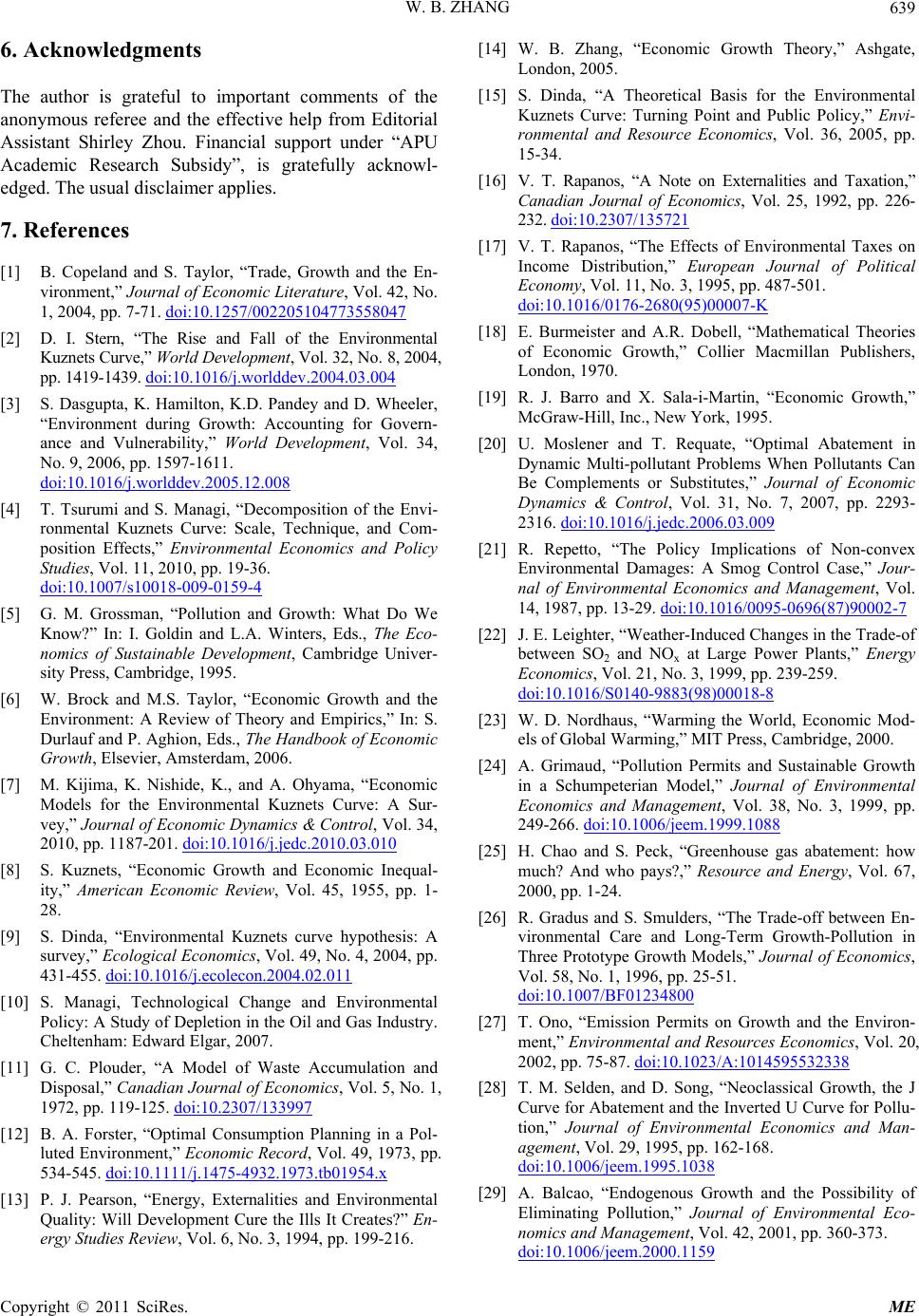

W. B. ZHANG639
6. Acknowledgments
The author is grateful to important comments of the
anonymous referee and the effective help from Editorial
Assistant Shirley Zhou. Financial support under “APU
Academic Research Subsidy”, is gratefully acknowl-
edged. The usual disclaimer applies.
7. References
[1] B. Copeland and S. Taylor, “Trade, Growth and the En-
vironment,” Journal of Economic Literature, Vol. 42, No.
1, 2004, pp. 7-71. doi:10.1257/002205104773558047
[2] D. I. Stern, “The Rise and Fall of the Environmental
Kuznets Curve,” World Development, Vol. 32, No. 8, 2004,
pp. 1419-1439. doi:10.1016/j.worlddev.2004.03.004
[3] S. Dasgupta, K. Hamilton, K.D. Pandey and D. Wheeler,
“Environment during Growth: Accounting for Govern-
ance and Vulnerability,” World Development, Vol. 34,
No. 9, 2006, pp. 1597-1611.
doi:10.1016/j.worlddev.2005.12.008
[4] T. Tsurumi and S. Managi, “Decomposition of the Envi-
ronmental Kuznets Curve: Scale, Technique, and Com-
position Effects,” Environmental Economics and Policy
Studies, Vol. 11, 2010, pp. 19-36.
doi:10.1007/s10018-009-0159-4
[5] G. M. Grossman, “Pollution and Growth: What Do We
Know?” In: I. Goldin and L.A. Winters, Eds., The Eco-
nomics of Sustainable Development, Cambridge Univer-
sity Press, Cambridge, 1995.
[6] W. Brock and M.S. Taylor, “Economic Growth and the
Environment: A Review of Theory and Empirics,” In: S.
Durlauf and P. Aghion, Eds., The Handbook of Economic
Growth, Elsevier, Amsterdam, 2006.
[7] M. Kijima, K. Nishide, K., and A. Ohyama, “Economic
Models for the Environmental Kuznets Curve: A Sur-
vey,” Journal of Economic Dynamics & Control, Vol. 34,
2010, pp. 1187-201. doi:10.1016/j.jedc.2010.03.010
[8] S. Kuznets, “Economic Growth and Economic Inequal-
ity,” American Economic Review, Vol. 45, 1955, pp. 1-
28.
[9] S. Dinda, “Environmental Kuznets curve hypothesis: A
survey,” Ecological Economics, Vol. 49, No. 4, 2004, pp.
431-455. doi:10.1016/j.ecolecon.2004.02.011
[10] S. Managi, Technological Change and Environmental
Policy: A Study of Depletion in the Oil and Gas Industry.
Cheltenham: Edward Elgar, 2007.
[11] G. C. Plouder, “A Model of Waste Accumulation and
Disposal,” Canadian Journal of Economics, Vol. 5, No. 1,
1972, pp. 119-125. doi:10.2307/133997
[12] B. A. Forster, “Optimal Consumption Planning in a Pol-
luted Environment,” Economic Record, Vol. 49, 1973, pp.
534-545. doi:10.1111/j.1475-4932.1973.tb01954.x
[13] P. J. Pearson, “Energy, Externalities and Environmental
Quality: Will Development Cure the Ills It Creates?” En-
ergy Studies Review, Vol. 6, No. 3, 1994, pp. 199-216.
[14] W. B. Zhang, “Economic Growth Theory,” Ashgate,
London, 2005.
[15] S. Dinda, “A Theoretical Basis for the Environmental
Kuznets Curve: Turning Point and Public Policy,” Envi-
ronmental and Resource Economics, Vol. 36, 2005, pp.
15-34.
[16] V. T. Rapanos, “A Note on Externalities and Taxation,”
Canadian Journal of Economics, Vol. 25, 1992, pp. 226-
232. doi:10.2307/135721
[17] V. T. Rapanos, “The Effects of Environmental Taxes on
Income Distribution,” European Journal of Political
Economy, Vol. 11, No. 3, 1995, pp. 487-501.
doi:10.1016/0176-2680(95)00007-K
[18] E. Burmeister and A.R. Dobell, “Mathematical Theories
of Economic Growth,” Collier Macmillan Publishers,
London, 1970.
[19] R. J. Barro and X. Sala-i-Martin, “Economic Growth,”
McGraw-Hill, Inc., New York, 1995.
[20] U. Moslener and T. Requate, “Optimal Abatement in
Dynamic Multi-pollutant Problems When Pollutants Can
Be Complements or Substitutes,” Journal of Economic
Dynamics & Control, Vol. 31, No. 7, 2007, pp. 2293-
2316. doi:10.1016/j.jedc.2006.03.009
[21] R. Repetto, “The Policy Implications of Non-convex
Environmental Damages: A Smog Control Case,” Jour-
nal of Environmental Economics and Management, Vol.
14, 1987, pp. 13-29. doi:10.1016/0095-0696(87)90002-7
[22] J. E. Leighter, “Weather-Induced Changes in the Trade-of
between SO2 and NOx at Large Power Plants,” Energy
Economics, Vol. 21, No. 3, 1999, pp. 239-259.
doi:10.1016/S0140-9883(98)00018-8
[23] W. D. Nordhaus, “Warming the World, Economic Mod-
els of Global Warming,” MIT Press, Cambridge, 2000.
[24] A. Grimaud, “Pollution Permits and Sustainable Growth
in a Schumpeterian Model,” Journal of Environmental
Economics and Management, Vol. 38, No. 3, 1999, pp.
249-266. doi:10.1006/jeem.1999.1088
[25] H. Chao and S. Peck, “Greenhouse gas abatement: how
much? And who pays?,” Resource and Energy, Vol. 67,
2000, pp. 1-24.
[26] R. Gradus and S. Smulders, “The Trade-off between En-
vironmental Care and Long-Term Growth-Pollution in
Three Prototype Growth Models,” Journal of Economics,
Vol. 58, No. 1, 1996, pp. 25-51.
doi:10.1007/BF01234800
[27] T. Ono, “Emission Permits on Growth and the Environ-
ment,” Environmental and Resources Economics, Vol. 20,
2002, pp. 75-87. doi:10.1023/A:1014595532338
[28] T. M. Selden, and D. Song, “Neoclassical Growth, the J
Curve for Abatement and the Inverted U Curve for Pollu-
tion,” Journal of Environmental Economics and Man-
agement, Vol. 29, 1995, pp. 162-168.
doi:10.1006/jeem.1995.1038
[29] A. Balcao, “Endogenous Growth and the Possibility of
Eliminating Pollution,” Journal of Environmental Eco-
nomics and Management, Vol. 42, 2001, pp. 360-373.
doi:10.1006/jeem.2000.1159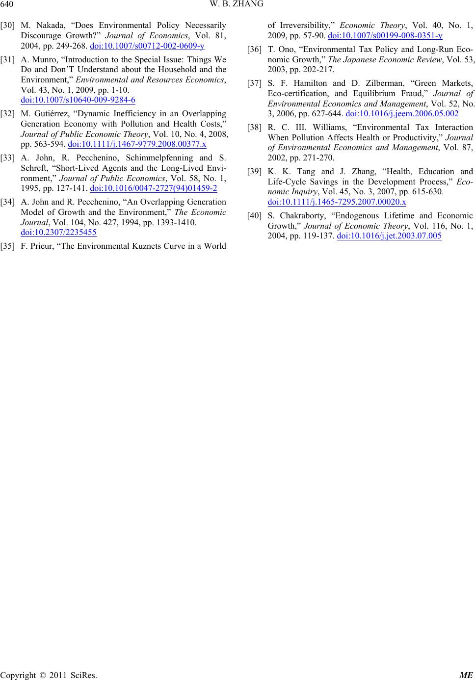

W. B. ZHANG 640
[30] M. Nakada, “Does Environmental Policy Necessarily
Discourage Growth?” Journal of Economics, Vol. 81,
2004, pp. 249-268. doi:10.1007/s00712-002-0609-y
[31] A. Munro, “Introduction to the Special Issue: Things We
Do and Don’T Understand about the Household and the
Environment,” Environmental and Resources Economics,
Vol. 43, No. 1, 2009, pp. 1-10.
doi:10.1007/s10640-009-9284-6
[32] M. Gutiérrez, “Dynamic Inefficiency in an Overlapping
Generation Economy with Pollution and Health Costs,”
Journal of Public Economic Theory, Vol. 10, No. 4, 2008,
pp. 563-594. doi:10.1111/j.1467-9779.2008.00377.x
[33] A. John, R. Pecchenino, Schimmelpfenning and S.
Schreft, “Short-Lived Agents and the Long-Lived Envi-
ronment,” Journal of Public Economics, Vol. 58, No. 1,
1995, pp. 127-141. doi:10.1016/0047-2727(94)01459-2
[34] A. John and R. Pecchenino, “An Overlapping Generation
Model of Growth and the Environment,” The Economic
Journal, Vol. 104, No. 427, 1994, pp. 1393-1410.
doi:10.2307/2235455
[35] F. Prieur, “The Environmental Kuznets Curve in a World
of Irreversibility,” Economic Theory, Vol. 40, No. 1,
2009, pp. 57-90. doi:10.1007/s00199-008-0351-y
[36] T. Ono, “Environmental Tax Policy and Long-Run Eco-
nomic Growth,” The Japanese Economic Review, Vol. 53,
2003, pp. 202-217.
[37] S. F. Hamilton and D. Zilberman, “Green Markets,
Eco-certification, and Equilibrium Fraud,” Journal of
Environmental Economics and Management, Vol. 52, No.
3, 2006, pp. 627-644. doi:10.1016/j.jeem.2006.05.002
[38] R. C. III. Williams, “Environmental Tax Interaction
When Pollution Affects Health or Productivity,” Journal
of Environmental Economics and Management, Vol. 87,
2002, pp. 271-270.
[39] K. K. Tang and J. Zhang, “Health, Education and
Life-Cycle Savings in the Development Process,” Eco-
nomic Inquiry, Vol. 45, No. 3, 2007, pp. 615-630.
doi:10.1111/j.1465-7295.2007.00020.x
[40] S. Chakraborty, “Endogenous Lifetime and Economic
Growth,” Journal of Economic Theory, Vol. 116, No. 1,
2004, pp. 119-137. doi:10.1016/j.jet.2003.07.005

W. B. ZHANG 641
Appendix
We now show that the dynamics can be expressed by a
two-dimensional differential equations system. From (2)
and (13), we obtain
,
i
ee
i
K
N
z
K
N
  (A1)
where we omit time index and /
ei ei



 By (A1)
and (8), we solve
,
11
ie
zK K
KK
zz


, (A2)
,
ie
zN N
NN
zz

.




(A3)
From e wN Y
e

 in (13) and (11), we have
ˆ
eii cwk
wN
F
NyNw rK  

 .
where we use ˆ cy

. Insert the definition of in the
above equation
ˆ y

,
ecwwii c
kc k
NNNwF K
rK
 

 






(A4)
where 1
kk

  and 1
ww



. Substituting (2)
into (A4) yields

0
0,
ei
cw wi
ii
ic k
ii
NNN
Ni
K
K
FK

 

 





 


(A5)
in which 1
ii

  and 0kc k

   Substitut-
ing (1), (A2) and (A3) into (A5), we solve
 
 
1/
0
0
,,
1
i
i
ii
ck
Az N
KzE z
z



 


  
 

(A6)
where
  

0
0
1
1.
ii ii cww
iii
zz
zz

  


 

We express K as a function of


zt and


Et. From
(A2), i
K
and e
K
are functions of z. From (A3), i
and e are functions of z. By the following procedure,
we can express other variables as functions of
N
N


zt and


Et at any point of time: i
F
by (1) → r and w by (2)
→e
Q by (10) → by (3) → c and s by (11). By these
results and from (9) we get the following differential
equation
ˆ
y








  
0
,
.
e
fi ce
Etzt Et
F
tCtQtE  
 


t
(A7)
We do not provide explicit expressions of the func-
tions as it is straightforward to do so and the expressions
are too tedious. Taking derivatives of (A9) with respect
to t yields
,
e
Kz
zE






 (A8)
where we also use (A7). Multiplying the two sides of (11)
with N and using (5), we have


ˆ,,
K
Ny zEK  
 (A9)
where we use (5). From (A8) and (A9), we solve
 
1
ˆ
,, .

ze
zzENyzEKEz 

   
 



 

(A10)
We have thus proved Lemma 1.
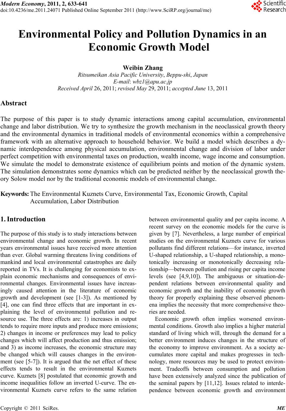