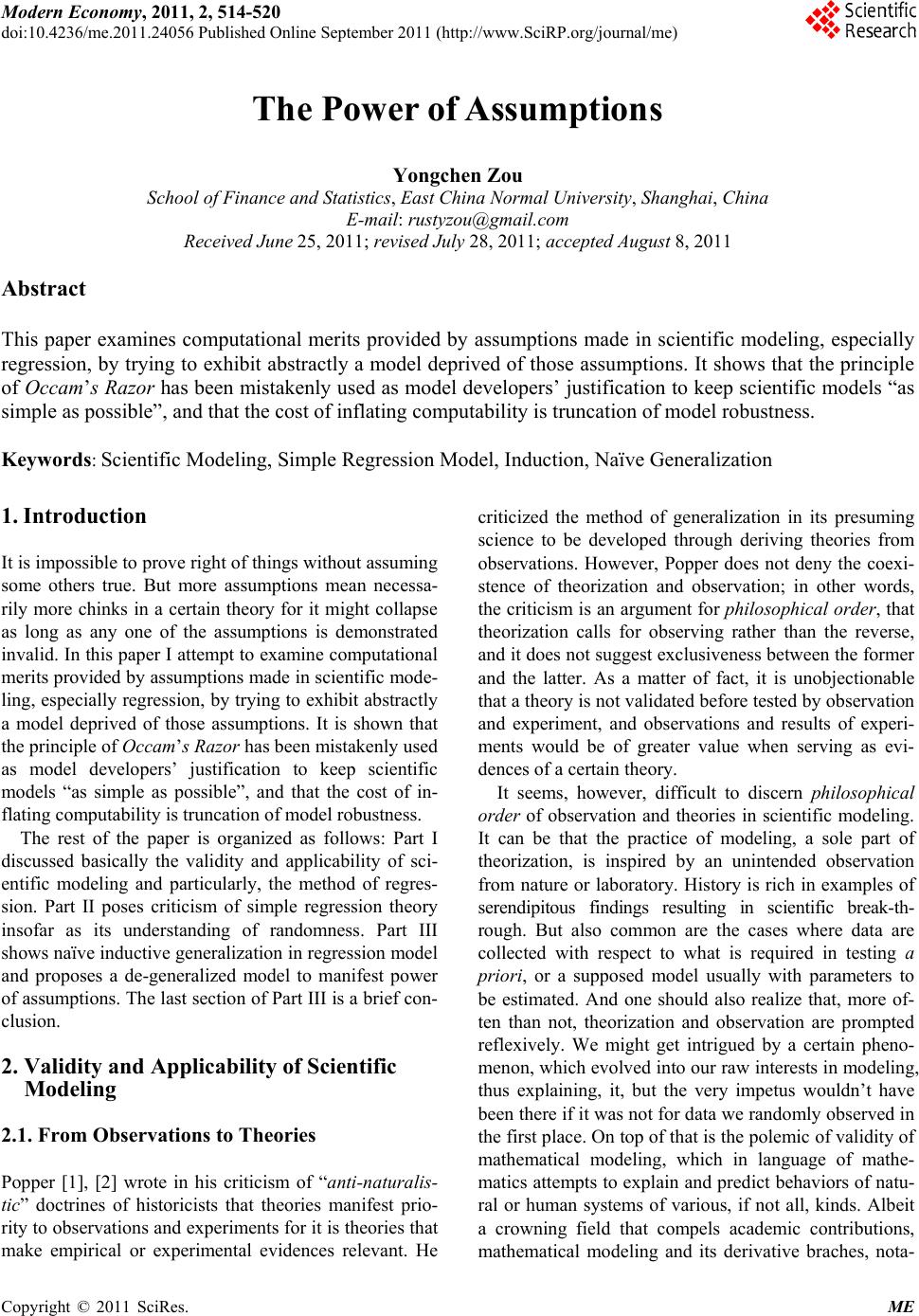Modern Economy, 2011, 2, 514-520
doi:10.4236/me.2011.24056 Published Online September 2011 (http://www.SciRP.org/journal/me)
The Power of Assumptions
Yongchen Zou
School of Finance and St at i stics, East China Normal University, Shanghai, China
Received June 25, 2011; revised July 28, 2011; accepted August 8, 2011
Abstract
This paper examines computational merits provided by assumptions made in scientific modeling, especially
regression, by trying to exhibit abstractly a model deprived of those assumptions. It shows that the principle
of Occam’s Razor has been mistakenly used as model developers’ justification to keep scientific models “as
simple as possible”, and that the cost of inflating computability is truncation of model robustness.
Keywords: Scientific Modeling, Simple Regression Model, Induction, Naïve Generalization
1. Introduction
It is impossible to prove right of things without assuming
some others true. But more assumptions mean necessa-
rily more chinks in a certain theory for it might collapse
as long as any one of the assumptions is demonstrated
invalid. In this paper I attempt to examine computational
merits provided by assumptions made in scientific mode-
ling, especially regression, by trying to exhibit abstractly
a model deprived of those assumptions. It is shown that
the principle of Occam’s Razor has been mistakenly used
as model developers’ justification to keep scientific
models “as simple as possible”, and that the cost of in-
flating computability is truncation of model robustness.
The rest of the paper is organized as follows: Part I
discussed basically the validity and applicability of sci-
entific modeling and particularly, the method of regres-
sion. Part II poses criticism of simple regression theory
insofar as its understanding of randomness. Part III
shows naïve inductive generalization in regression model
and proposes a de-generalized model to manifest power
of assumptions. The last section of Part III is a brief con-
clusion.
2. Validity and Applicability of Scientific
Modeling
2.1. From Observations to Theories
Popper [1], [2] wrote in his criticism of “anti-naturalis-
tic” doctrines of historicists that theories manifest prio-
rity to observations and experiments for it is theories that
make empirical or experimental evidences relevant. He
criticized the method of generalization in its presuming
science to be developed through deriving theories from
observations. However, Popper does not deny the coexi-
stence of theorization and observation; in other words,
the criticism is an argument for philosophical order, that
theorization calls for observing rather than the reverse,
and it does not suggest exclusiveness between the former
and the latter. As a matter of fact, it is unobjectionable
that a theory is not validated before tested by observation
and experiment, and observations and results of experi-
ments would be of greater value when serving as evi-
dences of a certain theory.
It seems, however, difficult to discern philosophical
order of observation and theories in scientific modeling.
It can be that the practice of modeling, a sole part of
theorization, is inspired by an unintended observation
from nature or laboratory. History is rich in examples of
serendipitous findings resulting in scientific break-th-
rough. But also common are the cases where data are
collected with respect to what is required in testing a
priori, or a supposed model usually with parameters to
be estimated. And one should also realize that, more of-
ten than not, theorization and observation are prompted
reflexively. We might get intrigued by a certain pheno-
menon, which evolved into our raw interests in modeling,
thus explaining, it, but the very impetus wouldn’t have
been there if it was not for data we randomly observed in
the first place. On top of that is the polemic of validity of
mathematical modeling, which in language of mathe-
matics attempts to explain and predict behaviors of natu-
ral or human systems of various, if not all, kinds. Albeit
a crowning field that compels academic contributions,
mathematical modeling and its derivative braches, nota-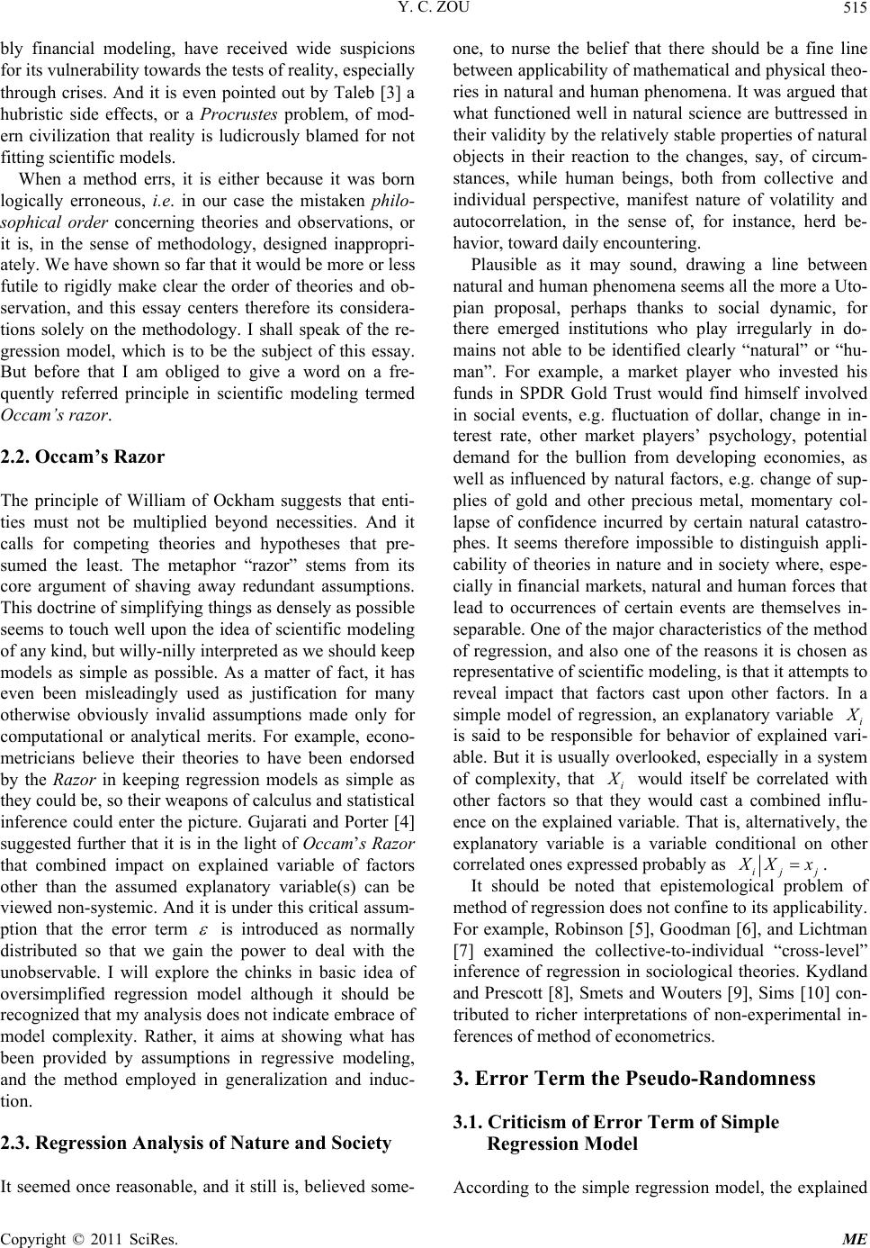

Y. C. ZOU515
bly financial modeling, have received wide suspicions
for its vulnerability towards the tests of reality, especially
through crises. And it is even pointed out by Taleb [3] a
hubristic side effects, or a Procrustes problem, of mod-
ern civilization that reality is ludicrously blamed for not
fitting scientific models.
When a method errs, it is either because it was born
logically erroneous, i.e. in our case the mistaken philo-
sophical order concerning theories and observations, or
it is, in the sense of methodology, designed inappropri-
ately. We have shown so far that it would be more or less
futile to rigidly make clear the order of theories and ob-
servation, and this essay centers therefore its considera-
tions solely on the methodology. I shall speak of the re-
gression model, which is to be the subject of this essay.
But before that I am obliged to give a word on a fre-
quently referred principle in scientific modeling termed
Occam’s razor.
2.2. Occam’s Razor
The principle of William of Ockham suggests that enti-
ties must not be multiplied beyond necessities. And it
calls for competing theories and hypotheses that pre-
sumed the least. The metaphor “razor” stems from its
core argument of shaving away redundant assumptions.
This doctrine of simplifying things as densely as possible
seems to touch well upon the idea of scientific modeling
of any kind, but willy-nilly interpreted as we should keep
models as simple as possible. As a matter of fact, it has
even been misleadingly used as justification for many
otherwise obviously invalid assumptions made only for
computational or analytical merits. For example, econo-
metricians believe their theories to have been endorsed
by the Razor in keeping regression models as simple as
they could be, so their weapons of calculus and statistical
inference could enter the picture. Gujarati and Porter [4]
suggested further that it is in the light of Occam’s Razor
that combined impact on explained variable of factors
other than the assumed explanatory variable(s) can be
viewed non-systemic. And it is under this critical assum-
ption that the error term

is introduced as normally
distributed so that we gain the power to deal with the
unobservable. I will explore the chinks in basic idea of
oversimplified regression model although it should be
recognized that my analysis does not indicate embrace of
model complexity. Rather, it aims at showing what has
been provided by assumptions in regressive modeling,
and the method employed in generalization and induc-
tion.
2.3. Regression Analysis of Nature and Society
It seemed once reasonable, and it still is, believed some-
one, to nurse the belief that there should be a fine line
between applicability of mathematical and physical theo-
ries in natural and human phenomena. It was argued that
what functioned well in natural science are buttressed in
their validity by the relatively stable properties of natural
objects in their reaction to the changes, say, of circum-
stances, while human beings, both from collective and
individual perspective, manifest nature of volatility and
autocorrelation, in the sense of, for instance, herd be-
havior, toward daily encountering.
Plausible as it may sound, drawing a line between
natural and human phenomena seems all the more a Uto-
pian proposal, perhaps thanks to social dynamic, for
there emerged institutions who play irregularly in do-
mains not able to be identified clearly “natural” or “hu-
man”. For example, a market player who invested his
funds in SPDR Gold Trust would find himself involved
in social events, e.g. fluctuation of dollar, change in in-
terest rate, other market players’ psychology, potential
demand for the bullion from developing economies, as
well as influenced by natural factors, e.g. change of sup-
plies of gold and other precious metal, momentary col-
lapse of confidence incurred by certain natural catastro-
phes. It seems therefore impossible to distinguish appli-
cability of theories in nature and in society where, espe-
cially in financial markets, natural and human forces that
lead to occurrences of certain events are themselves in-
separable. One of the major characteristics of the method
of regression, and also one of the reasons it is chosen as
representative of scientific modeling, is that it attempts to
reveal impact that factors cast upon other factors. In a
simple model of regression, an explanatory variable i
X
is said to be responsible for behavior of explained vari-
able. But it is usually overlooked, especially in a system
of complexity, that i
X
would itself be correlated with
other factors so that they would cast a combined influ-
ence on the explained variable. That is, alternatively, the
explanatory variable is a variable conditional on other
correlated ones expressed probably as ij
X
j
Xx
.

It should be noted that epistemological problem of
method of regression does not confine to its applicability.
For example, Robinson [5], Goodman [6], and Lichtman
[7] examined the collective-to-individual “cross-level”
inference of regression in sociological theories. Kydland
and Prescott [8], Smets and Wouters [9], Sims [10] con-
tributed to richer interpretations of non-experimental in-
ferences of method of econometrics.
3. Error Term the Pseudo-Randomness
3.1. Criticism of Error Term of Simple
Regression Model
According to the simple regression model, the explained

Y. C. ZOU 516
variable is expressed as a linear function of ex-
planatory
Y
X
by
01
YbbX

  (1)
where 0 is the intercept parameter and 1 the slope
parameter measuring sensitiveness of behavior of Y
with accordance to that of
b b
X
.

is the error term re-
sponsible for any factors other than
X
that affects Y
under the assumption that

is normally distributed
with mean zero or

0E   (2)
In practice the only work for the model assumer is to
have the two parameters well estimated, under observa-
tions of , with mathematical technique termed
Least Squares (LS), given by the equations

,
ii
YX

11 11
02
1
11
11
1
1
nn nn
iiii i
nii ii
inn
i
ii
ii
X
XXY
nn
bY
nnX X
n
 






 
 






 


Y



(3)
11 1
12
11
11
1
nn n
iii
ii i
nn
ii
ii
i
X
XY Y
nn
b
XX
n
 






 






 




(4)
Subtract the error

, which is a stochastic term, from
equation (1) we get the regression function geometrically
sketched as a line shaped with intercept 0 and slope
1. From equation (3) and (4) of Least Squares estimator
technique it is shown that value of and 1
b are de-
termined exclusively by observations i
. In other
words, shape of the regression function is determined by
data . But one should be
aware of the fact that estimates of intercept and slope
parameters are tenable only for a given set of data. That
is, so long as another arbitrary observation is added to
the initial data, computational values of 0
b and 1
should be revised to what is derived by equation (3) and
(4) with substituted by
b

,
i
YX
b
0
b
,
i
X

  
11 11
,, ,,
ii
YX YXYX

11 11
,,,,,YX YXY
 

,,
b

i



11 1111i
, and they are,
except for some rare cases, very unlikely to assume the
values they used to do.
,,,, ,,
ii i
YXXY

,Y,XYX
I suggest what this means to the method of regression
is ironical because a regression model is supposed to
reflect the relationship between behaviors of explanatory
and explained variables by means of determining 0 b
and 1. However, analysis above has just shown that the
shape of the regression function is determined not by the
true bond between and
b
Y
X
, but by the availability of
data. In real studies, however, we are not always confi-
dent about neither reliability nor completeness of the
data we obtain.
We may also look at what is said about the error term

. It is also called “disturbance” of regression for it at-
tempts to explain the non-systemic deviation of data
from the regression line. But this terminology seems to
contradict the definition, and I would attribute this error
to the confounded understanding of concepts of func-
tional-relationship model and regression model. A func-
tional-relationship model is buttressed usually by axioms
and ironclad theorems, whereas a regression model is
backed by a theory far from being indubitably proved.
Consider modeling the area of a given circle by

2
πSR


 (5)
where denotes the area of the circle, is the ob-
served radius and
SR

the non-systemic error incurred by
minor impacts of other factors like temperature and
gauging error. In a functional-relationship model as this,
the error term is justified to be termed “disturbance” for
factors other than observed radius is proved negligibly
weak in affecting the area. Yet when we think of a re-
gression model that regresses height against weight of an
individual, it is insecure to assert variables other than
weight are of minor significance for unlike equation (5),
functional-relationship between height and weight of
human beings is far from a rigorously proved theorem.
Another tricky argument for normality of the error
term is given by statistical advantage of the central limit
theorem. Because there are too many factors affecting
the explained variable, their mean impact is then accord-
ing to central limit theorem asymptocally normally dis-
tributed. This is a misleading conclusion for first, the
theorem can be proved tenable by using moment gene-
rating technique only for large number, but one in de-
veloping a regression model is not bestowed with the
priori of exactly how much factors other than the arbi-
trarily assumed independent variable are affecting the
dependent variable (otherwise those influences would be
incorporated into the model if one attempts to keep the
model reasonable and efficient), thus it is unjustifiable to
assert other factors to be “too many”. Second, central
limit theorem is developed upon a sheer probabilistic and
numerical premise. Random variables, whatever distri-
bution they have, are of no superior significance to each
other. In a large size sample composed of random vari-
ables of various distributions, one with normal distribu-
tion is of no greater impact than one with gamma. Cen-
tral limit theorem in this sense is not significance-
weighted. This is remarkably untrue for regression model
in that real life factors are always in different superiority
in explaining a certain end. For example, the depressive
impact on stock prices of a natural disaster in the short
run, we learned from history, is usually more eminent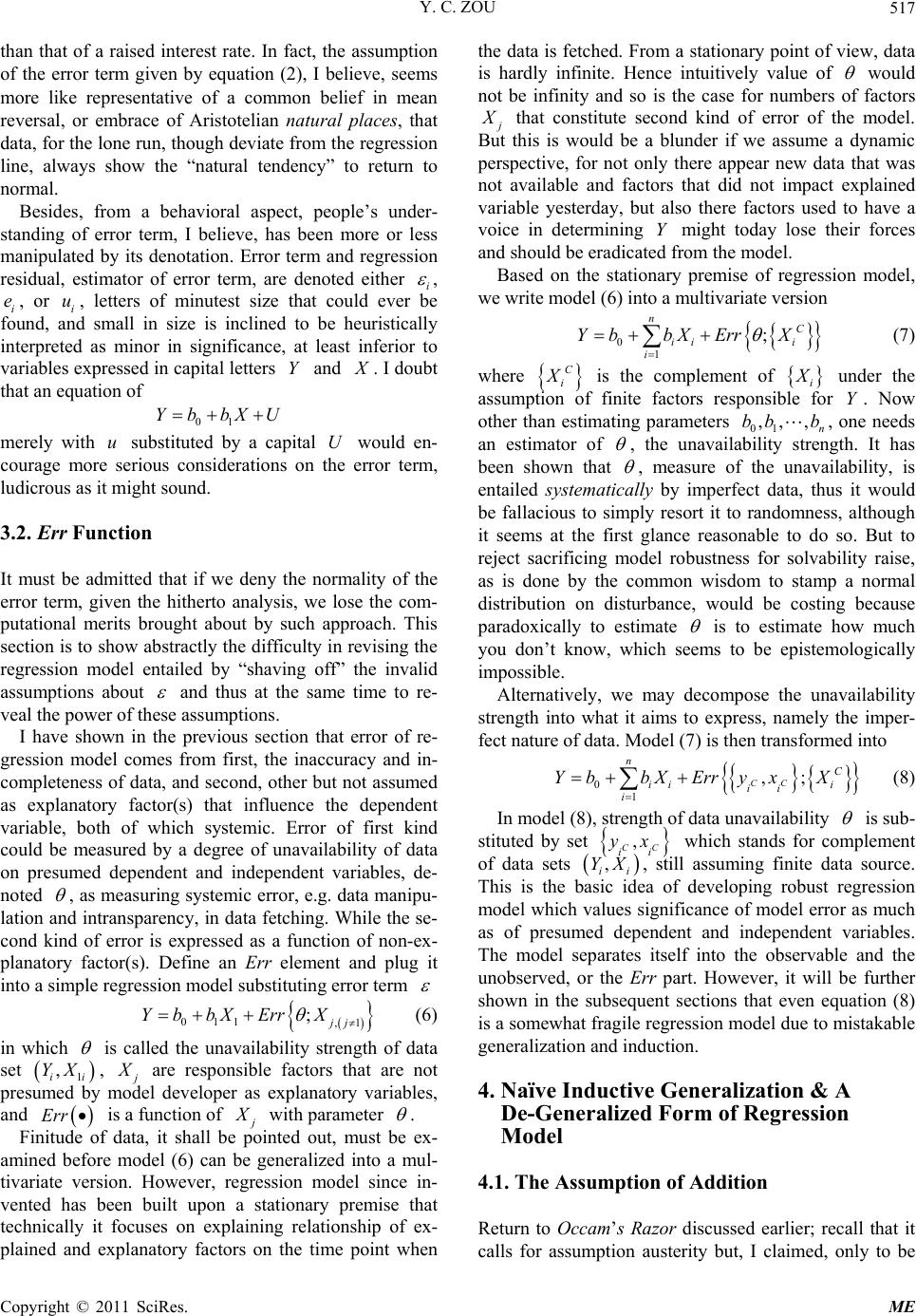

Y. C. ZOU517
than that of a raised interest rate. In fact, the assumption
of the error term given by equation (2), I believe, seems
more like representative of a common belief in mean
reversal, or embrace of Aristotelian natural places, that
data, for the lone run, though deviate from the regression
line, always show the “natural tendency” to return to
normal.
Besides, from a behavioral aspect, people’s under-
standing of error term, I believe, has been more or less
manipulated by its denotation. Error term and regression
residual, estimator of error term, are denoted either i

,
i, or i, letters of minutest size that could ever be
found, and small in size is inclined to be heuristically
interpreted as minor in significance, at least inferior to
variables expressed in capital letters and
e u
Y
X
. I doubt
that an equation of
01
YbbXU 
merely with substituted by a capital U would en-
courage more serious considerations on the error term,
ludicrous as it might sound.
u
3.2. Err Function
It must be admitted that if we deny the normality of the
error term, given the hitherto analysis, we lose the com-
putational merits brought about by such approach. This
section is to show abstractly the difficulty in revising the
regression model entailed by “shaving off” the invalid
assumptions about

and thus at the same time to re-
veal the power of these assumptions.
I have shown in the previous section that error of re-
gression model comes from first, the inaccuracy and in-
completeness of data, and second, other but not assumed
as explanatory factor(s) that influence the dependent
variable, both of which systemic. Error of first kind
could be measured by a degree of unavailability of data
on presumed dependent and independent variables, de-
noted

, as measuring systemic error, e.g. data manipu-
lation and intransparency, in data fetching. While the se-
cond kind of error is expressed as a function of non-ex-
planatory factor(s). Define an Err element and plug it
into a simple regression model substituting error term



011 ,1
;jj YbbX ErrX 

 

(6)
in which

is called the unavailability strength of data
set ,

1i
,
i
YX
j
X
are responsible factors that are not
presumed by model developer as explanatory variables,
and


Err  is a function of
j
X
with parameter

.
Finitude of data, it shall be pointed out, must be ex-
amined before model (6) can be generalized into a mul-
tivariate version. However, regression model since in-
vented has been built upon a stationary premise that
technically it focuses on explaining relationship of ex-
plained and explanatory factors on the time point when
the data is fetched. From a stationary point of view, data
is hardly infinite. Hence intuitively value of

would
not be infinity and so is the case for numbers of factors
j
X
that constitute second kind of error of the model.
But this is would be a blunder if we assume a dynamic
perspective, for not only there appear new data that was
not available and factors that did not impact explained
variable yesterday, but also there factors used to have a
voice in determining Y might today lose their forces
and should be eradicated from the model.
Based on the stationary premise of regression model,
we write model (6) into a multivariate version


0
1
;
nC
ii i
i
YbbX ErrX 

 
 
(7)
where


C
i
X is the complement of

i
X
under the
assumption of finite factors responsible for Y. Now
other than estimating parameters 01, one needs
an estimator of
,, ,
n
bbb

, the unavailability strength. It has
been shown that

, measure of the unavailability, is
entailed systematically by imperfect data, thus it would
be fallacious to simply resort it to randomness, although
it seems at the first glance reasonable to do so. But to
reject sacrificing model robustness for solvability raise,
as is done by the common wisdom to stamp a normal
distribution on disturbance, would be costing because
paradoxically to estimate

is to estimate how much
you don’t know, which seems to be epistemologically
impossible.
Alternatively, we may decompose the unavailability
strength into what it aims to express, namely the imper-
fect nature of data. Model (7) is then transformed into



0
1
,;
CC
nC
ii i
ii
i
YbbXErryxX

 
 (8)
In model (8), strength of data unavailability

is sub-
stituted by set


,
CC
i
yx
i
which stands for complement
of data sets


,
ii
YX , still assuming finite data source.
This is the basic idea of developing robust regression
model which values significance of model error as much
as of presumed dependent and independent variables.
The model separates itself into the observable and the
unobserved, or the Err part. However, it will be further
shown in the subsequent sections that even equation (8)
is a somewhat fragile regression model due to mistakable
generalization and induction.
4. Naïve Inductive Generalization & A
De-Generalized Form of Regression
Model
4.1. The Assumption of Addition
Return to Occam’s Razor discussed earlier; recall that it
calls for assumption austerity but, I claimed, only to be

Y. C. ZOU 518
falsely interpreted as “keep things as simple as possible”.
This can be seen in, for example, the very common prac-
tice that equates “and” to “add”. In regressive modeling,
if behavior of 1
X
and 2
X
are believed to be responsi-
ble for change in , then it is speculated that
Y
 
1122
YfX fX

  (9)
Computational benefits allowed by addition are re-
lentless. For example, one is free of the concern of com-
mutativity that may otherwise engrained in exponentia-
tion of model (9) for
 


11 2222 11
f
XfXfXfX
while does not necessarily equate


22
11
fX
fX


11
22
f
X
fX . To put it differently, one does not, thanks
to commuativity of addition, need to worry about the
order in which one arranges variables in his model. This
assumption of addition, as is illustrated, is taken as the
core intuitive knowledge of regression as well as a great
many other scientific models. It is consistent with the
misunderstood principle of the razor insofar as it man-
ages to “keep regression as simple as possible” in the
sense of mathematical easiness, although admittedly it
does circumvent unnecessary errors, in our case of (9),
that might be given rise by other mathematical opera-
tions, for example, multiplication. If model (9) is alterna-
tively speculated as

112 2
YfXfX

 (10)
then in a case where negative impact by both indepen-
dent variables 1
X
and 2
X
jointing into a magnified
positive impact upon , then it would be a major mis-
take.
Y
There are notwithstanding other operations that may
under specific problems superior than addition. The pre-
vious mentioned example of could have
been model of better realistic merit in modeling problem
of influence of interest rate and catastrophe events upon
stock market indices for taking chronological fact into
account. One should also be aware that operations that
might fit into a situation should not confine to those al-
ready in existence. Or, it could be not only unary, binary,
and functional operations, but also algebraic method that
is not yet invented but might come into exist, let’s ab-
stractly denote it “”, in the future.


22
11
fX
fX
21
?input input
4.2. De-Generalized Regression Model
It is readily seen that the generalization of simple regres-
sion model 011 YbbX

  to its multivariate version
01122 nn
YbbXbX bX

  (11)
is a progress of naïve induction under the unjustified
assumption of addition. Problems with this inductive
generalization, as is illustrated throughout this paper, are
first, a mistakable approach of cowardly resorting lack of
knowledge to randomness; second, an overlook of a pre-
sumed major assumption of taking a mathematical op-
eration for granted. To show ultimately the power of
these assumptions, I shall try to propose a rough idea of
what a robust model immune to naïve inductive gener-
alization looks like.
For our analysis does not confine to regression model
linear in parameter, it is preferable to present parameters
as functions


ii
f
b. But due to clarification of denota-
tion, we shall distinguish function of parameter and
function of variable so that i
X
in the model appears to
be


ii
F
X, hence we write











 






0001 11122
11 2
22
3
?? ???
?? ??
,;
CC
2
p
vp
nnn nn
pnp nv
C
i
ii
Yfb fbFXfb
FXfb FX
Err yxX


v
(12)
where = explained variable, Y
1,, n
X
X = assumed explanatory variables,
the question mark

= the mathematical op-
eration, invented or uninvented, before parameter
?ip
th
i

iv = the mathematical operation, invented or
uninvented, before variable
?th i
0 at the beginning of the expression is installed to
avoid the paradox that the equation itself is begin with a
“
?
0

”


,
CC
yx
ii
= complementary of obtained data, stand-
ing for incompleteness, given finitude of data


C
i
X = complementary of

1,, n

X
X, other
variables that have explanatory force but not presumed
as explanatory variables in the regression model, given
finitude of variables
At the cost of suffering from grand vagueness and
major decrease in computational convenience, Model (12)
eradicates a) naïvete of assuming addition, b) two kinds
of error mentioned in Part II on the error term. However,
careful inspection would make you find that model (12)
simply replace “

” with “

ip ” and “” with “

iv ” in
expression (11), thus although it no longer assumes sim-
ple operation of addition and multiplication of elements,
it is still not free from the assumption of addition unless
it takes into account impact of a) autocorrelation of vari-
ables, and b) chronological order of variables, or in its
essence, significance weight of variables.
? ?
Improvement a) could be achieved by condition a vari-
able upon precedent one(s), rewrite equation (12) into














  

00
0011
001 1
0001111 112
22,22 11 23
,,
111 1
??? ?
??
??
,,?, ;
nn
CC
bb pvp
bbbbvp
nnbb bb
np nv
C
nnnnni
ii
Yfb fbFX
fbFXXx
fb
FXXxXxErry xX












(13)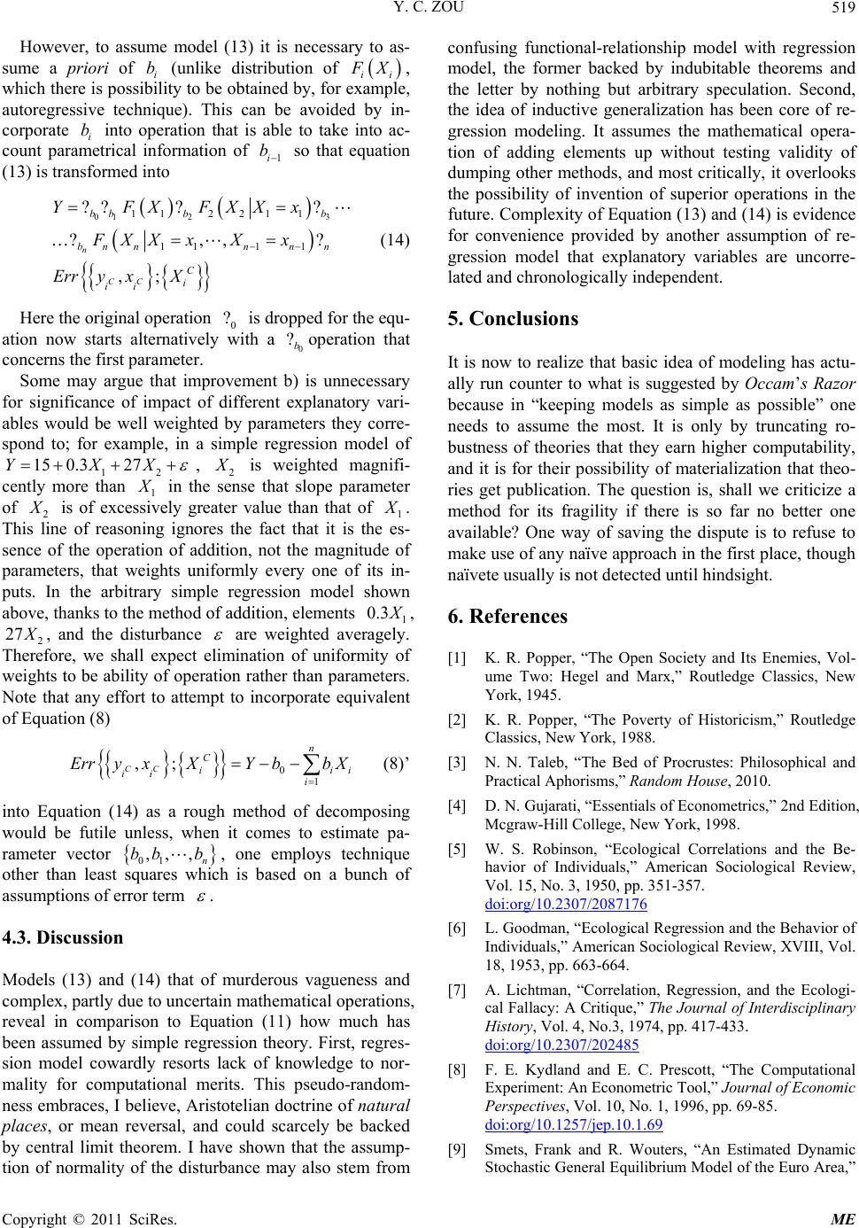

Y. C. ZOU519
However, to assume model (13) it is necessary to as-
sume a priori of i (unlike distribution of b


ii
F
X,
which there is possibility to be obtained by, for example,
autoregressive technique). This can be avoided by in-
corporate i into operation that is able to take into ac-
count parametrical information of so that equation
(13) is transformed into
b
1i
b





 

01 23
112211
111 1
?? ??
?,,
,;
n
CC
bb bb
bn nnnn
C
i
ii
YFXFXXx
FXXxXx
Err yxX






?

(14)
Here the original operation 0 is dropped for the equ-
ation now starts alternatively with a operation that
concerns the first parameter.
?
0
?b
Some may argue that improvement b) is unnecessary
for significance of impact of different explanatory vari-
ables would be well weighted by parameters they corre-
spond to; for example, in a simple regression model of
12
15 0.327YXX

 , 2
X
is weighted magnifi-
cently more than 1
X
in the sense that slope parameter
of 2
X
is of excessively greater value than that of 1
X
.
This line of reasoning ignores the fact that it is the es-
sence of the operation of addition, not the magnitude of
parameters, that weights uniformly every one of its in-
puts. In the arbitrary simple regression model shown
above, thanks to the method of addition, elements 1 0.3
X
,
2
27
X
, and the disturbance

are weighted averagely.
Therefore, we shall expect elimination of uniformity of
weights to be ability of operation rather than parameters.
Note that any effort to attempt to incorporate equivalent
of Equation (8)


 0
1
,;
CC
n
C
i
ii i
ErryxXYbb X


i i

(8)’
into Equation (14) as a rough method of decomposing
would be futile unless, when it comes to estimate pa-
rameter vector

01 , one employs technique
other than least squares which is based on a bunch of
assumptions of error term
,, ,
n
bb b

.
4.3. Discussion
Models (13) and (14) that of murderous vagueness and
complex, partly due to uncertain mathematical operations,
reveal in comparison to Equation (11) how much has
been assumed by simple regression theory. First, regres-
sion model cowardly resorts lack of knowledge to nor-
mality for computational merits. This pseudo-random-
ness embraces, I believe, Aristotelian doctrine of natural
places, or mean reversal, and could scarcely be backed
by central limit theorem. I have shown that the assump-
tion of normality of the disturbance may also stem from
confusing functional-relationship model with regression
model, the former backed by indubitable theorems and
the letter by nothing but arbitrary speculation. Second,
the idea of inductive generalization has been core of re-
gression modeling. It assumes the mathematical opera-
tion of adding elements up without testing validity of
dumping other methods, and most critically, it overlooks
the possibility of invention of superior operations in the
future. Complexity of Equation (13) and (14) is evidence
for convenience provided by another assumption of re-
gression model that explanatory variables are uncorre-
lated and chronologically independent.
5. Conclusions
It is now to realize that basic idea of modeling has actu-
ally run counter to what is suggested by Occam’s Razor
because in “keeping models as simple as possible” one
needs to assume the most. It is only by truncating ro-
bustness of theories that they earn higher computability,
and it is for their possibility of materialization that theo-
ries get publication. The question is, shall we criticize a
method for its fragility if there is so far no better one
available? One way of saving the dispute is to refuse to
make use of any naïve approach in the first place, though
naïvete usually is not detected until hindsight.
6. References
[1] K. R. Popper, “The Open Society and Its Enemies, Vol-
ume Two: Hegel and Marx,” Routledge Classics, New
York, 1945.
[2] K. R. Popper, “The Poverty of Historicism,” Routledge
Classics, New York, 1988.
[3] N. N. Taleb, “The Bed of Procrustes: Philosophical and
Practical Aphorisms,” Random House, 2010.
[4] D. N. Gujarati, “Essentials of Econometrics,” 2nd Edition,
Mcgraw-Hill College, New York, 1998.
[5] W. S. Robinson, “Ecological Correlations and the Be-
havior of Individuals,” American Sociological Review,
Vol. 15, No. 3, 1950, pp. 351-357.
doi:org/10.2307/2087176
[6] L. Goodman, “Ecological Regression and the Behavior of
Individuals,” American Sociological Review, XVIII, Vol.
18, 1953, pp. 663-664.
[7] A. Lichtman, “Correlation, Regression, and the Ecologi-
cal Fallacy: A Critique,” The Journal of Interdisciplinary
History, Vol. 4, No.3, 1974, pp. 417-433.
doi:org/10.2307/202485
[8] F. E. Kydland and E. C. Prescott, “The Computational
Experiment: An Econometric Tool,” Journal of Economic
Perspectives, Vol. 10, No. 1, 1996, pp. 69-85.
doi:org/10.1257/jep.10.1.69
[9] Smets, Frank and R. Wouters, “An Estimated Dynamic
Stochastic General Equilibrium Model of the Euro Area,”

Y. C. ZOU 520
Journal of the European Economic Association, Vol. 1,
No. 5, 2003, pp. 1123-1175.
doi:org/10.1162/154247603770383415
[10] C. A. Sims, “But Economics Is Not an Experimental
Science,” Journal of Economic Perspectives, Vol. 24, No.
2, pp. 59-68. doi:org/10.1257/jep.24.2.59