Modern Economy, 2011, 2, 468-478
doi:10.4236/me.2011.24052 Published Online September 2011 (http://www.SciRP.org/journal/me)
Are Business Management Games a Suitable Tool for
Analyzing the Boundedly Rational Behavior of
Economic Agents?
Oliver Musshoff1, Norbert Hirschauer2, Philipp Hengel1
1Department for Agricultural Economics and Rural Development, Universität Göttingen, Göttingen, Germany
2Institute of Agricultural and Nutritional Sciences, Universität Halle-Wittenberg, Halle (Saale), Germany
Received June 13, 20 11; revised July 14, 2011; accepted July 25, 2011
Abstract
Regulatory policies often aim to steer the behavior of economic agents by changing their economic environ-
ment. Assessing the potential impacts of regulatory policies requires forecasts regarding how humans adapt
to such changes. One important prerequisite for meaningful policy impact analysis is in-depth knowledge of
why and to what extent economic agents behave in a boundedly rational way. We propose that business
management games can be used to contribute towards better understanding of agent behaviors, since they
provide an inexpensive opportunity to reach beyond existing anecdotal evidence concerning “behavioral
anomalies”. Modifying an existing business management game in which investment, financing and produc-
tion decisions have to be made, we demonstrate how bounded rationality can be quantified and separated into
its two components: incomplete information and limited cognitive abilities. The resulting data show that de-
cisions made by participants in this game are strongly influenced by bounded rationality. They also show that
both incomplete information and limited cognitive abilities are relevant components of the bounded rationa-
lity displayed by players.
Keywords: Bounded Rationality, Business Management Games, Multi-Period Linear Programming, Policy
Impact Analysis
1. Introduction
Business (management) games have long been used to
familiarize students with the content of economic courses
[1-4]. As a byproduct of students’ learning, a large amount
of data accrues. With careful game design, high-quality
data can be obtained under controlled conditions and at
low cost. Economists should therefore consider exploiting
business games for both teaching and research.
Business management games are an especially promi-
sing tool to analyze decision making in general and to
examine whether and to what extent economic agents
make sub-optimal decisions in particular. Sub-optimal
decisions can be caused by incomplete information and/
or limited information-processing abilities. They can be
understood as a deviation from rational behavior in the
sense of inconsistency between individual goals and de-
cisions actually made by each individual. Simon [5] calls
this bounded ratio nality [6-7].
A number of social and political stakeholders are in-
terested in steering entrepreneurial behavior by changing
the economic environment. When assessing the likely
impacts of such policies, forecasts need to be made re-
garding the way economic agents adap t to such chang es.
In many cases political interventions are indeed linked
with the obligatio n to carry out an ex ante and an ex post
evaluation of results in term of behavioral changes and
impacts in terms of political goal achievement. A pro-
minent example is the EU Regulation on support for ru-
ral development (Council Regulation (EC) No 1698/
2005) and the corresponding Common Monitoring and
Evaluation Framework [8] which prescribe that all rural
development interventions are evaluated in order to gua-
rantee accountability and to assess the achievements of
the established political o bjectives.
Good forecasts require good understanding of entre-
preneurial decision-making [9]. As altered economic
conditions only affect micro-level decisions if they are

O. MUSSHOFF ET AL.469
actually perceived and considered in the planning pro-
cess, regulatory impact analysts need to take into account
the real character of economic agents, including their
bounded rationality. Otherwise, one runs the risk of de-
signing measures for economic agents who do not exist
in the real world.
A quick glance at regularly surveyed economic data
shows that there are significant differences in corporate
success. Let’s look at farming in Germany as an example.
During the financial year 2007/08 the return on equity of
the top third of arable farms of the national German farm
accountancy data network was higher by 13.7 percentage
points than that of the bottom third [10]. While this may
be taken as preliminary evidence that some economic
agents act less rational than others, the analysis of un-
controlled field data poses the general problem that it is
often very difficult or even impossible to isolate causal
relationships [11]. Besides the “degree of bounded ra-
tionality” both economic and natural situations may dif-
fer between agents. Simple examples of this are locally
or regionally differing prices for land of the same quality
and locally or regionally occurring damages (e.g., from
hailstorms, droughts). Furthermore, different agents may
pursue various other goals in addition to profit maximi-
zation such as financial security, free time or social
reputation. Due to these confounding elements the de-
gree of bounded rationality cannot be quantified based
on field data on corporate performance. To isolate the
effect of bounded rationality from such data, the per-
formance that could be achieved through rational beha-
vior would have to be known for each corporation. The
performance actually attained would then have to be
contrasted with this reference value. Such benchmarks
cannot be provided. Their derivation would require an
omniscient analyst who is able to factor in all idiosyn-
cratic specificities in an adequate way.
Methods for retrieving data to analyze decision be-
havior can be classified into five ideal types along a con-
tinuum of approaches: (1) collection of naturally occur-
ring field data, (2) collection of field data from random-
ized control trials, (3) collection of data through surveys
where interviewees are confronted with hypothetical de-
cision situations, (4) collection of data from business
management games, and (5) collection of data from labo-
ratory experiments. The ex ante, mid-term and ex post
evaluations carried out according to the above-mentioned
EU Regulation on support for rural development (Coun-
cil Regulation (EC) No 1698/2005) rely mainly on the
collection of naturally occurring field data. These evalua-
tions do not represent randomized control trials. The
changes of the economic environment, even though they
are “artificially” induced, are not systematically design ed
in order to generate knowledge. Instead they result from
practical political programs. Furthermore, even in ex ante
evaluations, surveys with hypothetical decision situation s,
business management games and laboratory experiments
are rarely used.
The controllability of contextual conditions and there-
fore internal validity in th e sense that observed cor- rela-
tions can be taken as causal relationships increases from
field data and surveys to management games and lab
experiments. In contrast, external validity in the sense
that observed relationships can be taken as being valid
for relevant real-life contexts decreases from one end of
the continuum to the other [12,11]. In laboratories, con-
ditions can almost completely be controlled and deliber-
ately varied [13]. For instance, one can determine almost
exactly how much time and what utilities are used by
participants and what forms of social communication are
permitted. While management games allow for margin-
ally less control, the essential characteristics of a de-
cision situation can still be purposefully designed ac-
cording to the researcher’s needs. Their great advantage
is furthermore that they can generate, as a by-product of
a pedagogical program, reliable and easily analyzable
data at very low cost.
Existing work on the q uantification o f bounded r ation-
ality usually resorts to surveys or lab experiments (for a
review [14]). Musshoff and Hirschauer [15] analyze the
magnitude of anomalies in hypothetical financing deci-
sions made by farmers via a survey. Sandri et al. [16] use
a lab experiment to examine whether decision makers
follow the real options approach or exhibit bounded ra-
tionality when confronted with disinvestment situations.
Gigliotti and Sopher [17] use experiments and confront
agents with a set of income streams, which have a clear
structure of dominance towards present-value income.
The experiments show, that a large percentage of agents
do not choose the payment stream that would maximize
their present-value income. Trip et al. [18] use informa-
tion matrices generated by specialized flower producers
in workshops to analyze whether these producers consis-
tently choose cultivars that fit their personal preferences.
This paper examines th e degree of bounded rationality
of students in an incentive-compatible multi-period and
multi-personal business management game. The game, in
which investment, financing and production decisions
have to be made, is about maximizing terminal wealth in
a competitive environment. That is, in contrast to most
lab experiments and surveys, which are restricted to very
simple partial problems, we were able to model a rela-
tively realistic decision situation. Using various norma-
tive benchmarks, we examine the relevance of incom-
plete information, on the one hand, and limited informa-
tion-processing capacities, on the other. To our know-
ledge, no existing work thus far has either explored the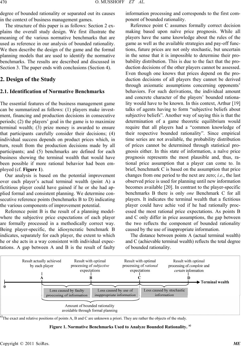

O. MUSSHOFF ET AL. 470
degree of bounded rationality or separated out its causes
in the context of business management games.
The structure of this p aper is as follows: Section 2 ex-
plains the overall study design. We first illustrate the
meaning of the various normative benchmarks that are
used as reference in our analysis of bounded rationality.
We then describe the design of the game and the formal
planning models that are used to identify the normative
benchmarks. The results are described and discussed in
Section 3. The pap er ends with c onclusions (Se ct i o n 4 ).
2. Design of the Study
2.1. Identification of Normative Benchmarks
The essential features of the business management game
can be summarized as follows: (1) players make invest-
ment, financing and production decisions in consecutive
periods; (2) the players’ goal in the game is to maximize
terminal wealth; (3) prize money is awarded to ensure
that participants carefully consider their decisions; (4)
individual success depends on product prices which, in
turn, result from the production decisions made by all
participants; and (5) benchmarks are defined for each
business showing the terminal wealth that would have
been possible if more rational behavior had been em-
ployed (cf. Figure 1).
Our analysis is based on the potential improvement
over each player’s actual terminal wealth (point A) a
fictitious player could have gained if he or she had ap-
plied formal and consistent planning. We determine con-
secutive reference points (benchmarks B to D) indicating
the various components of improvement potential.
Reference point B is the result of a planning model-
where the subjective price expectations of each player
are formally processed in a methodically correct way.
Being player-specific, the idiosyncratic benchmark B
indicates, separately for each player, the extent to which
he or she acts in a way consistent with individual expec-
tations. A gap between A and B is the result of faulty
information processing and corresponds to the first com-
ponent of bounded rationality.
Reference point C assumes formally correct decision
making based upon naïve price prognosis. While all
players have the same knowledge about the rules of the
game as well as the available strategies and pay-off func-
tions, future prices are not only stochastic, but uncertain
in the sense that it is impossible to determine their pro-
bability distribution. This is due to the fact that the pro-
duction decisions of the other players cannot be assessed.
Even though one knows that prices depend on the pro-
duction decisions of all players they cannot be derived
through axiomatic assumptions concerning opponents’
behaviors. For such derivations, the individual amount
and concrete character of the players’ bounded rationa-
lity would have to be known. In this context, Arthur [19]
talks of agents having to form “subjective beliefs about
subjective beliefs”. Anoth er way of saying this is that the
determination of a game theoretic equilibrium would
require that all players had a “common knowledge of
their respective bounded rationality”. Since empirical
time series are not available, the probability distribution
of prices cannot be determined through statistical pro-
gnosis either. In this state of information, a naïve price
prognosis represents the most plausible and, thus, ra-
tional price assumption that a player can come to. In
brief, benchmark C is based on the assumption that price
changes from one period to the next are zero; i.e., the last
observed price is used for planning until new information
becomes available [20]. In contrast to the player-specific
benchmarks B there is only one Benchmark C for all
players. It indicates the terminal wealth that a fictitious
player could have achie ved if he had rationally proc-
essed the most rational price expectations. As points B
and C only differ in price assumptions, the gap between
the two reflects the component of bounded rationality
caused by the use o f inappropriate information.
The distance between points A (actual terminal wealth)
and C (achiev able ter minal w ealth ) reflec ts th e total d egree
of bounded rationality.
a)The exact and relative positions of points A, B and C are unknown a priori. They are rather the ob jects of the study.
Figure 1. Normative Benchmarks Used to Analyze Bounded Rationality. a)

O. MUSSHOFF ET AL. 471
In Figure 1, we have positioned point A to the left of
benchmark B, and benchmark B to the left of benchmark
C. This is not necessarily the case for all players. On the
one hand, a player’s price prognosis could accidentally
be better than the naïve prognosis. Then, point B would
have to be positioned to the right of point C. On the other
hand, better subjective price predictions or “lucky” com-
binations of inappropriate price predictions and faulty
information processing could lead to even better results
than correct processing of appropriate price forecasts. In
such cases, players would be right for the wrong reasons.
Just a s a gambler h as a chance of winning even th e most
improbable bets, a player may achieve a better result
with boundedly rational behavior than through a system-
atic approach. If this is the case for a particular player,
point A will lie to the right of point C. The question
whether and to what extent points A, B and C differ from
each other is the subject matter of our study.
It should be noted that point D is the result of a model
based not only on rational price expectations but unreal-
istically on certain information. That is, the production
decisions of the other game participants are assumed to
be a priori knowledge of one fictitious player. Hence,
benchmark D can neither be beaten by actual players nor
by other benchmarks. It represents an “unfair” reference
since forecasts cannot be made with certainty neither in
our business management game nor in reality. This is
why point D is used on ly for a relative positioning of the
actual results and the other benchmarks.
It should furthermore be noted that points B, C and D
denote strategies which we label “individual” because
they are based on the perspective that one fictitious
player without influencing the game’s market price1
adopts the respective strategy. A “collective” perspective
(which we do not adopt) would imply that all players
adopt the strategy. While coinciding with the equilibrium
approach [21-22] often used in economic analysis, the
collective perspective is not useful when looking for
normative benchmarks in the game that is actually
played. Benchmark C, for instance, denotes the optimal
strategy for a fictitious player who knows that he is
playing a game with a group of boundedly rational play-
ers (cf. Table 1). Adopting the collective perspective
would only yield a useful decision rule if, and only if, it
were realistic to assume that the bounded rationality of
all players were completely eliminated by learning (ca-
pacity building) or by competition. But then we would
no longer need to explor e bounded rationality.
Table 1. Individual vs. Collective Perspective in the Case of
Benchmark C.
Individual perspective Collective perspective
Type of
reference
point
Success of a fictitious actor
playing the optimal
strategy.
Identical success of all
players playing the optimal
strategy.
Assumption Co-players act boundedly
rational. All players act rationally.
2.2. Description of the Game
2.2.1. Desi gn
We use a modified version of the business management
game “Sparrow or Pigeon”, which was developed for
teaching purposes by Brandes [21]. The most important
modification is that we offer prize money to ensure in-
centive compatibility. Each participant controls a busi-
ness for which he or she has to decide on investments,
finance and production in eight consecutive periods. De-
cisions have to be made weekly. Before getting started
for good, players have the opportunity to play one learn-
ing round in order to get acquainted with the game.
The starting situation at the beginning of period 1 is
identical for all players: everybody has a starting capital
of 2,000 monetary units (MU), and everybody has the
same set of entrepreneurial choices. Nobody owns any
production facilities yet. Two production activities, spa-
rrows and pigeons, can be chosen. The price for sparrows
(in MU/piece) is deterministic and known to every-
body:
S
t
p
13.5,if1,2,3,4
12.0,if 5,6,7,8
S
t
t
pt




(1)
Due to a presumed demand shock for birds it is re-
duced after period 4

t. Future pigeon prices are
uncertain. They depend on aggregate pigeon production.
In each period
p
t
p
,
t
the following linear demand function
applies:
,
1
1
max 0;250.14N
PP
tt
n
px
N




n
(2)
In equation (2) is the number of players partici-
pating in the game and the number of pigeons pro-
duced by player The size of the market i s proporti onal
to the number of players originally participating in the
game. Thus, in different game cycles with different num-
bers of starting players, the same price is achieved if the
average pigeon production per player remains the same.
Stock-keeping is not possible. That is, the production of a
period has to be sold at the price valid in that period.
N
.
Pnt
x,
n
Players can choose between five types of discrete in-
vestments to build up prod uction capacities (cf. Table 2).
Production facilities differ in terms of purchase value,
1Even though the number of players is relatively small in our game, the
p
roduction decision of one player has only a marginal effect on prices.
This “price-taker-structure” is in line with the structure of many real
markets where the market shares of competing players are too small to
have a noticeable effect on prices.

O. MUSSHOFF ET AL. 472
Table 2. Overview of Investment Alternatives.
Production capacitya) Variable costs (MU/unit)
Investment
alternative Purchase
value (MU) Sparrows Pigeons
Useful life
(periods) Sparrows Pigeons
Lending limit
(%)
A 70 20 (birds) 2 9 9 0
B 195 25 0 3 8 – 80
C 340 0 25 3 – 6 80
D 1,560 75 0 3 3 – 50
E 1,760 0 75 3 – 2 50
a)Maximum number of units producible in each period.
production capacity, useful life, and variable costs. Faci-
lity A uses a versatile technology that can be u sed for the
production of sparrows or pigeons the proportion of
which can be changed from one period to the next period.
Facilities B, C, D, and E are specialized for the produc-
tion of one or the other. Disinvestments are not possible;
that is, investment costs are completely sunk. Production
facilities are depreciated in a linear manner and entered
in the balance sheet at their book value. The determine-
stic price of sparrows exceeds their production costs.
Hence, there is a safe way to earn profits. Funds which
are not used for production purposes yield an interest rate
of 4% per period.
At the beginning of each period, players (businesses)
make their investments, determine their production pro-
gram and decide on how to finance their decisions. Fur-
thermore, every business has to pay 300 MU to the game
authority to account for fixed costs. At the end of each
period, the production is sold at the price according to
equation (1) and (2). Furthermore, debt services are due.
Subsequently, i.e., at the beginning of the next period,
each player may make new decisions.
Funding requirements can be met by accumulated liq-
uid funds (equity) or a maximum overdraft credit of
2,000 MU at an interest rate of 15% per period. In addi-
tion, the production facilities B, C, D, and E can be
partly financed by annuity loans at an interest rate of
10% per period. The players always have to be liquid. A
business is automatically retired from the game if it can-
not meet its payment obligations at the beginning of a
period.
The objective of the game is to accumulate the highest
terminal wealth by the end of period 8. To provide in-
centive compatibility, we announced the following prize
money: the five players with the highest terminal wealth
get 100 € (1st), 80 € (2nd), 60 € (3rd), 40 € (4th), or 20 €
(5th). The rank of players was not disclosed until th e end
of the game to prevent players from dropping out be-
cause of poor performance. Besides the prize money for
the top performers we also asked the players to make a
price prediction at the beginning of each round for the
following three periods. The best overall price prognosis
was rewar ded with 50 €.
2.2.2. Participants
The game was played twice without changing any of the
rules, once in the winter term of 2008/09 (group 1) and
once in the summer term of 2009 (group 2), with par-
ticipants being mostly students of agricultural science at
Göttingen University. In total, 105 participants were reg-
istered (58 in group 1, and 47 in group 2). Participants
who went bankrupt or did not participate during the
whole game for other reasons were not included in the
analysis, as benchmark B cannot be determined for these
individuals. Table 3 gives an overview of the play ers.
We were able to analyze 23 players in each group. On
average, participants in group 2 had been studying 1.2
terms longer than players in group 1. However, they as-
sessed their own economic abilities as being a little lower
than grou p 1 did.
Subsequent to the game, we asked the players which
utilities and decision criteria they had applied. Figure 2
gives an overview of the answers.
In this questioning more players (56) took part than w e
were able to include in the benchmark analysis (46), as
some players who had not participated during the whole
game nonetheless answered our questions.
The majority of the players used technical utilities
such as spreadsheet programs (66%) or calculators (55%).
About one fourth stated that they had made their deci-
sions based on a “gut feeling”. In addition, 45% con-
ducted a liquidity analysis. Furthermore, various meth-
ods of investment analysis were used for decision mak-
ing. Finally, 11% stated that they had used risk analysis
and linear programming models.
2.3. Description of the Normative Benchmark
Model
2.3.1. The Optimizing Model
We compare the results actually achieved by the players
in the game with normative benchmarks B, C and D (cf.
Figure 1). These benchmarks were calculated via a
mixed-integer multi-period linear programming model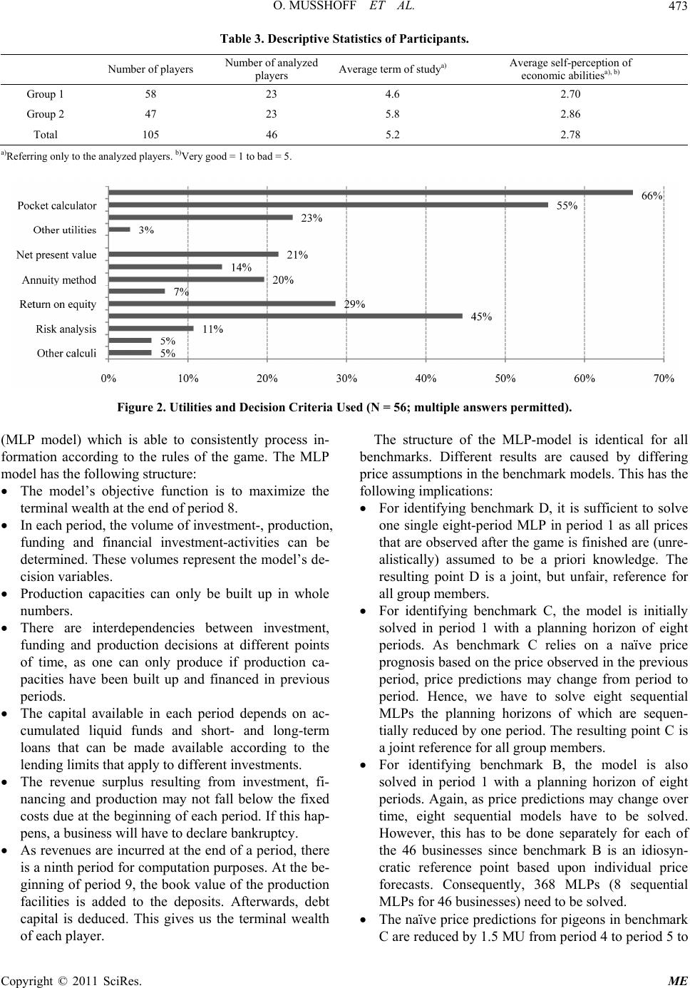

O. MUSSHOFF ET AL. 473
Table 3. Descriptive Statistics of Participants.
Number of players Number of analyzed
players Av erage term of studya) Average self-perception of
economic abilitiesa), b)
Group 1 58 23 4.6 2.70
Group 2 47 23 5.8 2.86
Total 105 46 5.2 2.78
a)Referring only to the analyzed players. b)Very good = 1 to bad = 5.
Figure 2. Utilities and Decision Criteria Used (N = 56; multiple answers permitted).
(MLP model) which is able to consistently process in-
formation according to the rules of the game. The MLP
model has the following structure:
 The model’s objective function is to maximize the
terminal wealth at the end of period 8.
 In each period, the volume of investment-, production,
funding and financial investment-activities can be
determined. These volumes represent the model’s de-
cision variables.
 Production capacities can only be built up in whole
numbers.
 There are interdependencies between investment,
funding and production decisions at different points
of time, as one can only produce if production ca-
pacities have been built up and financed in previous
periods.
 The capital available in each period depends on ac-
cumulated liquid funds and short- and long-term
loans that can be made available according to the
lending limits that apply to different investments.
 The revenue surplus resulting from investment, fi-
nancing and production may not fall below the fixed
costs due at the beginning of each period. If this hap-
pens, a business will have to declare bankruptcy.
 As revenues are incurred at the end of a period, there
is a ninth period for computation purposes. At the be-
ginning of p eriod 9, the book valu e of the production
facilities is added to the deposits. Afterwards, debt
capital is deduced. This gives us the terminal wealth
of each player.
The structure of the MLP-model is identical for all
benchmarks. Different results are caused by differing
price assumptions in the benchmark models. This has the
following implications:
 For identifying benchmark D, it is sufficient to solve
one single eight-period MLP in period 1 as all prices
that are observed after the game is finished are (unre-
alistically) assumed to be a priori knowledge. The
resulting point D is a joint, but unfair, reference for
all group members.
 For identifying benchmark C, the model is initially
solved in period 1 with a planning horizon of eight
periods. As benchmark C relies on a naïve price
prognosis based on the price observed in the previous
period, price predictions may change from period to
period. Hence, we have to solve eight sequential
MLPs the planning horizons of which are sequen-
tially reduced by one period. The resulting point C is
a joint reference for all group members.
 For identifying benchmark B, the model is also
solved in period 1 with a planning horizon of eight
periods. Again, as price predictions may change over
time, eight sequential models have to be solved.
However, this has to be done separately for each of
the 46 businesses since benchmark B is an idiosyn-
cratic reference point based upon individual price
forecasts. Consequently, 368 MLPs (8 sequential
MLPs for 46 businesses) need to be solved.
 The naïve price predictions for pigeons in benchmark
C are reduced by 1.5 MU from period 4 to period 5 to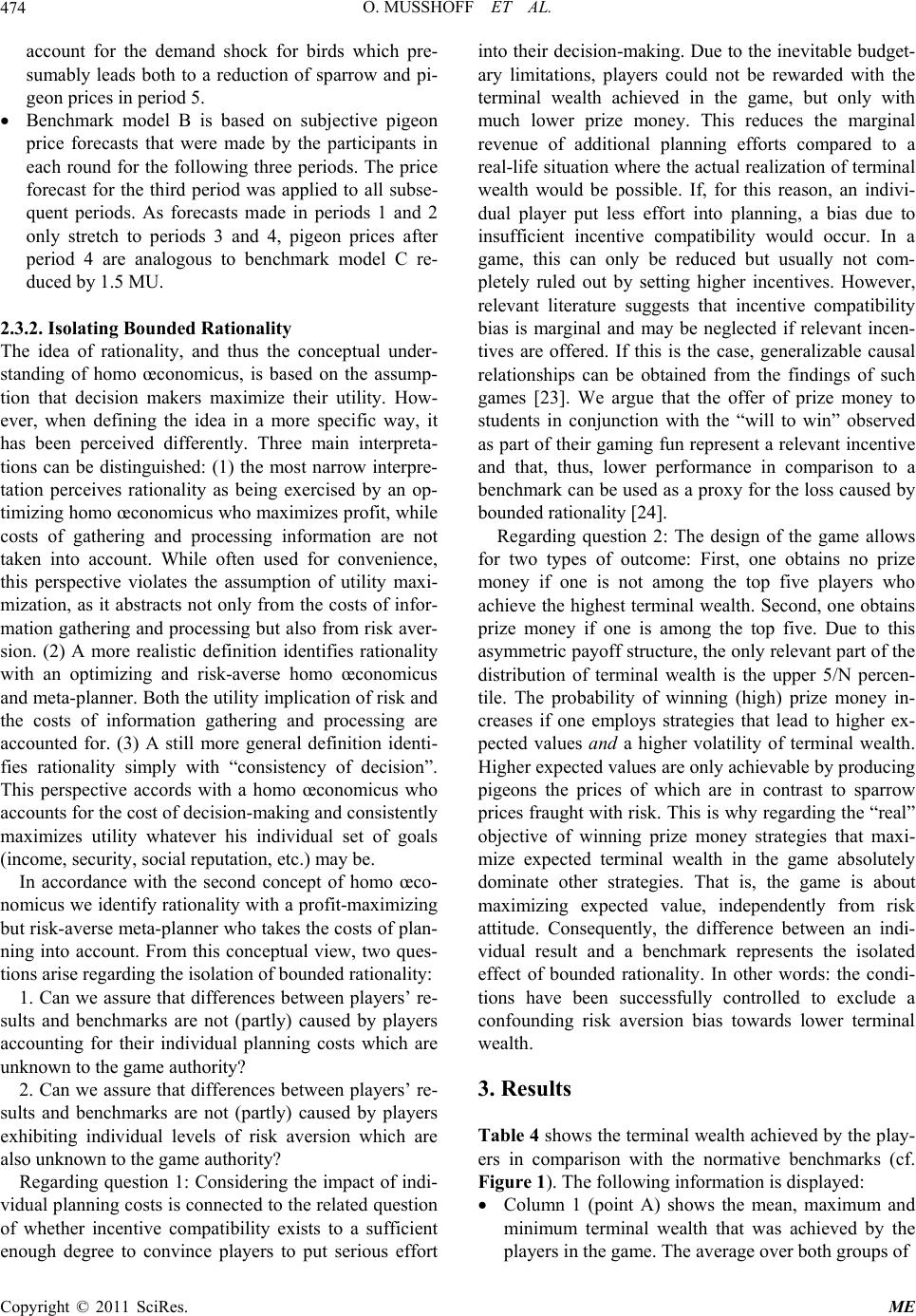

O. MUSSHOFF ET AL. 474
account for the demand shock for birds which pre-
sumably leads both to a reduction of sparrow and pi-
geon prices in period 5.
 Benchmark model B is based on subjective pigeon
price forecasts that were made by the participants in
each round for the following three periods. The price
forecast for the third period was applied to all subse-
quent periods. As forecasts made in periods 1 and 2
only stretch to periods 3 and 4, pigeon prices after
period 4 are analogous to benchmark model C re-
duced by 1.5 MU.
2.3.2. Isolating Bounded Rationality
The idea of rationality, and thus the conceptual under-
standing of homo œconomicus, is based on the assump-
tion that decision makers maximize their utility. How-
ever, when defining the idea in a more specific way, it
has been perceived differently. Three main interpreta-
tions can be distinguished: (1) the most narrow interpre-
tation perceives rationality as being exercised by an op-
timizing homo œconomicus who maximizes profit, while
costs of gathering and processing information are not
taken into account. While often used for convenience,
this perspective violates the assumption of utility maxi-
mization, as it abstracts not only from the costs of infor-
mation gathering and processing but also from risk aver-
sion. (2) A more realistic definition identifies rationality
with an optimizing and risk-averse homo œconomicus
and meta-planner. Both the utility implicat ion of risk and
the costs of information gathering and processing are
accounted for. (3) A still more general definition identi-
fies rationality simply with “consistency of decision”.
This perspective accords with a homo œconomicus who
accounts for the cost of decision-making and consistently
maximizes utility whatever his individual set of goals
(income, security, social reputation, etc.) may be.
In accordance with the second concept of homo œco-
nomicus we identify rationality with a profit-maximizing
but risk-averse meta-planner who takes the costs of plan-
ning into account. From this conceptual view, two ques-
tions arise regarding the iso lation of bounded rationality:
1. Can we assure that differences between players’ re-
sults and benchmarks are not (partly) caused by players
accounting for their individual planning costs which are
unknown to the game authority?
2. Can we assure that differences between players’ re-
sults and benchmarks are not (partly) caused by players
exhibiting individual levels of risk aversion which are
also unknown to the game author ity?
Regarding question 1: Considering the impact of indi-
vidual planning costs is connected to the related question
of whether incentive compatibility exists to a sufficient
enough degree to convince players to put serious effort
into their decision-making. Due to the inevitable budget-
ary limitations, players could not be rewarded with the
terminal wealth achieved in the game, but only with
much lower prize money. This reduces the marginal
revenue of additional planning efforts compared to a
real-life situation where the actual realization of terminal
wealth would be possible. If, for this reason, an indivi-
dual player put less effort into planning, a bias due to
insufficient incentive compatibility would occur. In a
game, this can only be reduced but usually not com-
pletely ruled out by setting higher incentives. However,
relevant literature suggests that incentive compatibility
bias is marginal and may be neglected if relevant incen-
tives are offered. If this is the case, generalizable causal
relationships can be obtained from the findings of such
games [23]. We argue that the offer of prize money to
students in conjunction with the “will to win” observed
as part of their gaming fun represent a relevant incentive
and that, thus, lower performance in comparison to a
benchmark can be used as a proxy for the loss caused by
bounded rationality [24].
Regarding question 2: The design of the game allows
for two types of outcome: First, one obtains no prize
money if one is not among the top five players who
achieve the highest terminal wealth. Second, one obtains
prize money if one is among the top five. Due to this
asymmetric payoff structure, the only relevant part of the
distribution of terminal wealth is the upper 5/N percen-
tile. The probability of winning (high) prize money in-
creases if one employs strategies that lead to higher ex-
pected values and a higher volatility of terminal wealth.
Higher expected values are only achievable by producing
pigeons the prices of which are in contrast to sparrow
prices fraught with risk. This is why regarding the “real”
objective of winning prize money strategies that maxi-
mize expected terminal wealth in the game absolutely
dominate other strategies. That is, the game is about
maximizing expected value, independently from risk
attitude. Consequently, the difference between an indi-
vidual result and a benchmark represents the isolated
effect of bounded rationality. In other words: the condi-
tions have been successfully controlled to exclude a
confounding risk aversion bias towards lower terminal
wealth.
3. Results
Table 4 shows the terminal wealth achiev ed by the play-
ers in comparison with the normative benchmarks (cf.
Figure 1). The following information is displayed:
 Column 1 (point A) shows the mean, maximum and
minimum terminal wealth that was achieved by the
players in the game. The average over both groups of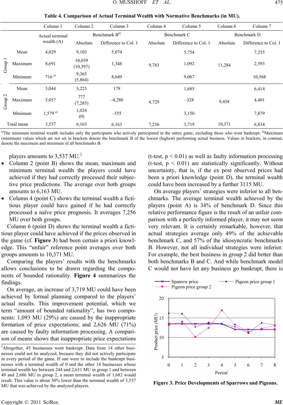

O. MUSSHOFF ET AL. 475
Table 4. Comparison of Actual Terminal Wealth with Normative Benchmarks (in MU).
Co l umn 1 Colum n 2 Column 3 Column 4 Column 5 Column 6 Column 7
Benchmark Bb) Ben chmark C Benchmark D
Actual terminal
wealth (A) Absolute Difference to Col. 1Absolute Difference to Col. 1Absolute Difference to Col. 1
Mean 4,029 9,103 5,074 5,754 7,255
Maximum 8,691 10,039
(10,397) 1,348 1,092 2,593
Group 1
Minimum 716 a) 9,365
(5,864) 8,649
9,783
9,067
11,284
10,568
Mean 3,044 3,223 179 1,685 6,414
Maximum 5,057 777
(7,285) –4,280 –328 4,401
Group 2
Minimum 1,579 a) 1,024
(0) –555
4,729
3,150
9,458
7,879
Total mean 3,537 6,163 6,163 7,256 3,719 10,371 6,834
a)The minimum terminal wealth includes only the participants who actively participated in the entire game, excluding those who went bankrupt; b)Maximum
(minimum) values which are not set in brackets denote the benchmark B of the lowest (highest) performing actual business. Values in brackets, in contrast,
denote the maximum and minimum of all benchmar k s B.
players amounts to 3,537 MU.2
 Column 2 (point B) shows the mean, maximum and
minimum terminal wealth the players could have
achieved if they had correctly processed their subjec-
tive price predictions. The average over both groups
amounts to 6,163 MU.
 Column 4 (point C) shows the terminal wealth a ficti-
tious player could have gained if he had correctly
processed a naïve price prognosis. It averages 7,256
MU over both groups.
Column 6 (point D) shows the terminal wealth a ficti-
tious player could have achieved if the prices observed in
the game (cf. Figure 3) had been certain a priori knowl-
edge. This “unfair” reference point averages over both
groups amounts to 10,371 MU.
Comparing the players’ results with the benchmarks
allows conclusions to be drawn regarding the compo-
nents of bounded rationality. Figure 4 summarizes the
findings.
On average, an increase of 3,719 MU could have been
achieved by formal planning compared to the players’
actual results. This improvement potential, which we
term “amount of bounded rationality”, has two compo-
nents: 1,093 MU (29%) are caused by the inappropriate
formation of price expectations; and 2,626 MU (71%)
are caused by faulty information processing. A compari-
son of means shows that inappropriate price expectations
(t-test, p < 0.01) as well as faulty information processing
(t-test, p < 0.01) are statistically significantly. Without
uncertainty, that is, if the ex post observed prices had
been a priori knowledge (point D), the terminal wealth
could have been increased by a further 3115 MU.
On average players’ strategies were inferior to all ben-
chmarks. The average terminal wealth achieved by the
players (point A) is 34% of benchmark D. Since this
relative performance figure is the result of an unfair com-
parison with a perfectly informed player, it may no t seem
very relevant. It is certainly remarkable, however, that
actual strategies average only 49% of the achievable
benchmark C, and 57% of the idiosyncratic benchmarks
B. However, not all individual strategies were inferior.
For example, the best business in group 2 did better than
both benchmarks B and C. And while benchmark model
C would not have let any business go bankrupt, there is
2Altogether, 45 businesses went bankrupt. Data from 14 other busi-
nesses could not be analyzed, because they did not actively participate
in every period of the game. If one were to include the bankrupt busi-
nesses with a terminal wealth of 0 and the other 14 businesses whose
terminal wealth lay between 244 and 2,631 MU in group 1 and between
49 and 2,686 MU in group 2, a mean terminal wealth of 1,682 would
result. This value is about 50% lower than the terminal wealth of 3,537
MU that was achieved by the analyzed players. Figure 3. Price Developments of Sparrows and Pigeons.

O. MUSSHOFF ET AL. 476
Figure 4. The Average Components of Bounded Rationality (in MU).
one case where an idiosyncratic benchmark strategy B
would have ruined a business, though the individual
player survived with his strategy. Absolute frequencies
show a similar picture: we find that benchmark strategy
B would have achieved better results than the players did
in 31 out of 46 cases. Benchmark strategy C would have
achieved better results in 44 out of 46 cases.
Much discussion has been devoted to the question of
whether bounded individual ration ality is still observable
on aggregate levels such as markets [14,25]. An alterna-
tive formulation of this question is whether markets be-
have in a rational way because the forces of competition
guarantee that market participants adopt rational behav-
ior. This question has gained much interest in the recent
regulatory debate about the financial crisis [26]. The ba-
sic question asked in this particular debate is whether
financial markets are efficient without regulation, or
whether the opposite is the case. While our simple busi-
ness management game is far from the complexities of
financial markets, it provides a feature that may be of
interest. We find that, as a result of competing players’
production decisions, pigeon prices oscillate around an
equilibrium price. Due to a sequence of individual over-
and under-reactions the market is far from equilibrium at
most times. That is, the equilibrium price is only very
rarely reached, and if so, only by chance. Market equi-
librium in our case (and perhaps in many real markets)
thus represents a “point attractor” similar to the station-
ary point of a clock pendulum which, if the clockwork is
wound up, is only transitorily touched. The pendulum
analogy implies that the understanding of market equi-
librium may be necessary but not sufficient to understand
and predict the decisions of boundedly rational actors
and the resulting market dynamics.
4. Conclusions
Nearly a decade ago, Trip et al. observed that it is still in
discussion whether games are suitable for research pur-
poses [18]. While being still valid, the question today
should more specifically be asked as to which games are
suitable for which research purposes. This question de-
marcates the starting point of our study which is aimed at
isolating the two components of bounded rationality: in-
complete information and limited information processing
abilities. For this purpose, the contextual conditions of
decision-making behavior have to be clearly controlled
to avoid confounding influences of uncontrolled vari-
ables. While this could be done in a lab experiment, we
investigated which potential a less costly business man-
agement game has for such an analysis. We found that
through careful design of the game we could con- trol the
conditions sufficiently to establish internal vali- dity and
answer the que s t i o n of interest .
Our multi-period and multi-personal business manage-
ment game relied upon a convenience sample of students
of agricultu ral science. The performance of these student
players was compared with normative benchmarks that
were consistently derived from formal planning models.
On average, we found that players’ performance was
reduced by more than 50% by bounded rationality. Over
70% of this loss, in turn, was caused by inconsistent in-
formation processing and nearly 30% by inappropriate
information. These findings represent additional empiri-
cal evidence that decision makers exhibit a substantial
amount of bounded rationality and that both of its com-
ponents, incomplete information and limited information
processing abilities, are relevant.
While producing internally valid results, the structure
of our business management game is, similarly to lab
experiments, devoid of many real-life complexities [27].
Furthermore, the players, being recruited from a conven-
ience sample of students, may exhibit other characteri-
stics than real-life actors who are of interest in a particu-
lar analysis. They may, for instance, exhibit a different

O. MUSSHOFF ET AL.477
degree or type of bounded rationality. External validity
thus being low, the results have to be interpreted with
caution and can only be tentatively generalized to other
populations and contexts.
We can make the general conclusion that, due to the
potential relevance of bounded rationality, rational-choice
models are not always adequate for assessing the beha-
vioral outcomes following changes in the economic en-
vironment. When searching for adequate models, regu-
latory impact analysts must therefore make a critical and
deliberate choice which accounts for bounded rationality
in all contexts where it exerts a significant influence on
behavior.
Identifying adequate models for regulatory impact
analysis is not easy, and the knowledge that decision
makers may act in boundedly rational ways does not
seem very helpful on first sight. This is due to the fact
that constructing a decision model, that closes the gap
between actual behavior and rational-choice prognoses
[28], would require to reconstruct the set of choices and
the calculi of individual agents. For this purpose, the
heterogeneity of agents in terms of their bounded indi-
vidual rationalities and assessments would need to be
taken into account. Usually, this kind of individual data
is either not available or prohibitively costly to come to.
Thus, the attempt to define a boundedly rational choice
model for each agent is out of question in most cases.
A feasible alternative may be to use context-specific
business management games with representative groups
of economic agents to simulate their boundedly rational
adaptation to novel environments. Games with represen-
tative groups of players can be seen as an intermediate
step between lab experiments and games with conven-
ience groups, on the one hand, and field experiments in
the form of randomized control trials, on the other. Such
a game simulation of expected behavioral adaptation has
two advantages. First, it provides an adequate combina-
tion of intern al and external validity: through an ap t con-
trol of conditions analysts can isolate behavioral effects
caused by the policy measures under investigation. Due
to the representativeness of the group, they are also able
to generalize the effects identified in the game to the
population of inter est. Second, g ames with rep resentativ e
groups provide the opportunity to carry out an ex ante
analysis of regulatory impacts. Such a prospective analy-
sis may safe tax payers’ money compared to econometric
analysis and conventional randomized control trials in
the field which represent an ex post evaluation after
costly policy measures have been implemented.
The use of context- and group-specific business man-
agement games seems especially attractive since the costs
of generating meaningful data are very low, both com-
pared to other methods and compared to the costs of in-
effective and erring policy measures. They exhibit a par-
ticular potential if the policies to be evaluated are novel,
i.e., if an econometric analysis of data observed from
past policy implementations and environmental condi-
tions does not “unveil” the agents’ preferences and
boundedly rational behaviors under changed environ-
ments. In other words, context- and group-specific games
may contribute towards less po litical measures being de-
signed and implemented for agents who in reality do not
exist.
Our study indicates that rational choice is not always
suitable for explaining economic decision-making. Two
research directions emerge from this finding: First, the
behavioral economic aspects of bounded ration ality need
to be researched more deep ly. This implies, for instance,
collecting information regarding the players’ socio-eco-
nomic background such as education, age, income, fam-
ily background, etc. It also implies investigating the de-
cision-making process in order to disclose the algorithms,
heuristics and calculi used in the decision. Second, a
systematic classification of real-life situations needs to
be developed, thus providing support to the political im-
pact analyst who has to make an adequate methodical
choice for the analysis of a particular policy. Such a sys-
tematization of situatio ns could start from the distinction
of two ideal-types: in highly competitive markets bound-
edly rational actors who are slow learners will rather
quickly be “competed out of the market”. In such cases,
rational-choice models are rather appropriate. In contrast,
in situations where competition and selection pressure
are low, there will be room for prolonged boundedly
rational behavior, the consequences of which can only be
analyzed adequately by methods which account for the
actors’ true characteristics. Sometimes the distinction may
not be unambiguous. In such cases, an adequate metho-
dical choice may involve combining rational-choice
models with context- and group-specific business man-
agement games.
5. Acknowledgements
The authors wo uld like to thank anonymous ref erees and
the editors for helpful comments and suggestions. We
gratefully acknowledge financial support from Deutsche
Forschungsgeme i nschaft (DFG).
6. References
[1] B. Keys and J. Wolfe, “The Role of Management Games
and Simulations in Education and Research,” Journal of
Management, Vol. 16, No. 2, 1990, pp. 307-336.
doi:org/10.1177/014920639001600205
[2] J. W. Longworth, “Management Games and the Teaching
of Farm Management,” Australian Journal of Agricu-

O. MUSSHOFF ET AL. 478
ltural Economics, Vol. 13, No. 1, 1969, pp. 58-67.
[3] J. W. Longworth, “From War-Chess to Farm Manag-
ment Games,” Canadian Journal of Agricultural Econo-
mics, Vol. 18, No. 2, 1970, pp. 1-11.
doi:org/10.1111/j.1744-7976.1970.tb00897.x
[4] C. Tanner, “A Survey of Students’ Attitudes to Methods
of Teaching Farm Management,” Australian Journal of
Agricultural Economics, Vol. 19, No. 1, 1975, pp. 52-62.
[5] H. A. Simon, “Rational Choice and the Structure of En-
vironments,” Psychological Review, Vol. 63, No. 2, 1956,
pp. 129-138. doi:org/10.1037/h0042769
[6] G. Gigerenzer and R. Selten, “Bounded Rationality: The
Adaptive Toolbox,” MIT Press, Cambridge, 2002.
[7] R. Selten, “Bounded Rationality,” Journal of Institutional
and Theoretical Economics, Vol. 146, No. 4, 1990, pp.
649-658.
[8] CMEF, “Common Monitoring and Evaluation Frame-
work,” Retrieved February 18, 2011.
http://ec.europa.eu/agriculture/rurdev/eval/index_en.htm.
[9] V. Smith, “Theory and Experiments: What are the Que-
stions?” Journal of Economic Behavior and Organization,
Vol. 73, No. 1, 2010, pp. 3-15.
doi:org/10.1016/j.jebo.2009.02.008
[10] BMELV, “Buchführungsergebnisse der Testbetriebe
2007/2008,” 2008.
http://www.bmelv-statistik.de/de/testbetriebsnetz/buchfue
hrungsergebnisse-landwirtschaft/#c1088
[11] B. E. Roe and D. R. Just, “Internal and External Validity
in Economics Research: Tradeoffs between Experiments,
Field Experiments, Natural Experiments and Field Data,”
American Journal of Agricultural Economics, Vol. 91,
No. 5, 2009, pp. 1266-1271.
doi:org/10.1111/j.1467-8276.2009.01295.x
[12] K. H. Coble, Z. Yang and M. D. Hudson, “Using Experi-
mental Economics to Evaluate Alternative Subjective
Elicitation Procedures,” Applied Econom i c s, 2009.
doi:org/10.1080/0003684080.
[13] D. Hudson, “Problem Solving and Hypothesis Testing
Using Economic Experiments,” Journal of Agricultural
and Applied Economics, Vol. 35, No. 2, 2003, pp. 337-
347.
[14] J. Conlisk, “Why Bounded Rationality?” Journal of Eco-
nomic Literature, Vol. 34, No. 2, 1996, pp. 669-700.
[15] O. Musshoff and N. Hirschauer, “A Behavioral Economic
Analysis of Bounded Rationality in Farm Financing Deci-
sions: First Empirical Evidence,” Agricultural Finance
Review, Vol. 71, No. 1, 2011, pp. 62-83.
[16] S. Sandri, C. Schade, O. Musshoff and M. Odening,
“Holding On for Too Long? An Experimental Study on
Inertia in Entrepreneurs’ and Non-Entrepreneurs’ Disin-
vestment Choices,” Journal of Economic Behavior and
Organization, Vol. 76, No. 1, 2010, pp. 30-44.
doi:org/10.1016/j.jebo.2010.02.011
[17] G. Gigliotti and B. Sopher, “Violations of Present-Value
Maximization in Income Choice,” Theory and Decision,
Vol. 43, No. 1, 1997, pp. 45-69.
doi:org/10.1023/A:1004950613488
[18] G. Trip, R. B. M. Huirne and J. A. Renkema, “Evaluating
Farmers’ Choice Processes in the Laboratory: Workshops
with Flower Producers,” Review of Agricultural Econo-
mics, Vol. 23, No. 1, 2001, pp. 185-201.
doi:org/10.1111/1058-7195.00054
[19] W. B. Arthur, “Inductive Reasoning and Bounded Ra-
tionality,” American Economic Review, Vol. 84, No. 2,
1994, pp. 406-411.
[20] H. Theil, “Applied Economic Forecasting,” Elsevier, Am-
sterdam, 1966.
[21] W. Brandes, “Über Selbstorganisation in Planspielen Ein
Erfahrungsbericht,” Schriften des Vereins für Socialpo-
litik, Gesellschaft für Wirtschafts-und Sozialwissen Sch-
aften, Neue Folge Band 195/VI, 2002, pp. 61-83.
[22] A. C. Hoggatt, “An Experimental Business Game,” Beha-
vioral Science, Vol. 4, No. 3, 1959, pp. 192-203.
[23] P. J. Schoemaker, “The Expected Utility Model: Its Vari-
ants, Purposes, Evidence and Limitations,” Journal of
Economic Literature, Vol. 20, No. 2, 1982, pp. 529-563.
[24] C. A. Holt, “Teaching Economics with Classroom Ex-
periments: A Symposium”, Southern Economic Journal,
Vol. 65, No. 3, 1999, pp. 603-610.
doi:org/10.2307/1060819
[25] B. S. Frey and R. Eichenberger, “Anomalies in Political
Economy,” Public Choice, Vol. 68, No. 1-3, 1991, pp.
71-89. doi:org/10.1007/BF00173820
[26] R. Skidelsky, “Keynes. The Return of the Master,” Pen-
guin, London, 2 009.
[27] A. Tversky and D. Kahneman, “Rational Choice and the
Framing of Decisions,” Rational Choice, University of
Chicago Press, Chicago, 1987, pp. 67-94.
[28] A. Rubinstein, “Comments on the Interpretation of Game
Theory, ” Econometrica, Vol. 59, No. 4, 1991, pp. 909-924.