 American Journal of Computational Mathematics, 2011, 1, 152-158 doi:10.4236/ajcm.2011.13017 Published Online September 2011 (http://www.SciRP.org/journal/ajcm) Copyright © 2011 SciRes. AJCM A Fourth Order Improved Numerical Scheme for the Generalized Burgers—Huxley Equation Athanassios G. Bratsos Department of Mathematics, Technological Educational Institution of Athens, Athens, Greece E-mail: bratsos@teiath.gr Received March 30, 2011; revised May 5, 2011; accepted May 22, 2011 Abstract A fourth order finite-difference scheme in a two-time level recurrence relation is proposed for the numerical solution of the generalized Burgers-Huxley equation. The resulting nonlinear system, which is analyzed for stability, is solved using an improved predictor-corrector method. The efficiency of the proposed method is tested to the kink wave using both appropriate boundary values and conditions. The results arising from the experiments are compared with the relevant ones known in the available bibliography. Keywords: Burgers-Huxley; Finite-Difference Method; Modified Predictor-Corrector 1. Introduction A. Hodgkin and A. Huxley [1] proposed a model, known henceforth as the Huxley equation, in order to explain the ionic mechanisms underlying the initiation and pro- pagation of action potentials in the squid giant axon. The most general form of the Huxley equation, known as the generalized Burgers-Huxley equation (BgH) [2,3], has the form [4] =1;0 1,>0 txxx uuuu uuuxt , (1.1) where is a sufficiently often differentiable function, =,uuxt a real parameter, 0 , and 0,1 >0 . Equation (1.1), which models the interaction be- tween reaction mechanisms, convection effects and dif- fusion transport, is the modified Burgers equation for =0 (see [5] and the references therein), is also the Huxley equation [1] for =0 , =1 and is the Fitz- hugh-Nagoma equation [6] for =0 . Many researchers have used various methods to solve the BgH equation. A theoretical study of the BgH equa- tion was found in Wang et al. [4], while analytical solu- tions using various techniques in [7-11], etc., have been proposed. As far as the numerical methods are concerned among others the Adomian decomposition method was used by Ismail et al. [12] for the BgH and the Bur- gers-Fisher equation, and by Hashim et al. [13] for the BgH equation. Javidi [14] used the pseudospectral me- thod, while Javidi [15], Javidi and Golbabai [16] the spectral collocation method. Batiha et al. [17] used the variational iteration method and Khattak [18] the collo- cation method with radial basis functions. Babolian and Saeidian [19] used the homotopy analysis method, etc. The initial condition associated with Equation (1.1) will be ,0=; 01.uxf xx (1.2) Theoretical Solution It is known [4] that Equation (1.1) has the following kink wave solution 1 ,= tanh 22 uxtkx ct (1.3) in which 241 =41 k and 2 14 =121 c 1 are the wave number and the velocity respectively. 2. The numerical Method 2.1. Development of the Method 2.1.1. Grid and Solution Vecto r To obtain numerical solutions the region =,Rxt 0< <10, T with its boundary consisting of R  A. G. BRATSOS 153 the lines , and is covered with a rectangular mesh of points, , with co-ordinates =0x=1x=0t G , t =, mn t n=,mh , mn with . The theoretical solution of Equation (1.1) at the typical mesh point =0,1, ,1mN t Ut will be denoted by and the relevant of an approximating difference scheme by . n m u n m U =n tt 1 , . n N U Let the solution vector at time level be 01 ,, n U ==U nn U (2.1) 2.1.2. Boundaries The following were used: 1) The space derivatives at the left boundary were replaced with second order finite-difference replace- ments of the form ([20] p. 17) =0x 2 n UU 2 has 01 4 nn =0 xx 1 =3 2 uU h0,h (2.2) 2 4 n U nd 1,u 0ash 2 3 n U 01 =tgt 01 5 nn =g 2 1 =2uU h 0,ut =0 xx xhU a (2.3) and with analogous replacements to the right boundary . =1x 2) The boundary conditions t (2.4) =0,1=0;u n > xx0,t =1 (2.5) were used, while at the other interior points of the grid G the well-known approximants based on the central-dif- ference formulas. 2.2. The Proposed Method Applying Equation (1.1) at each point of the grid G at time level ; leads to a first-order initial-value problem, which is written in a matrix-vector form as == n tt ,2,n 1 ,N tt fx U 0=0 , = Dt t UU = A fx UU 01 , Bt U= fx ;>0 f (2.6) in which =diagd dDt, == =d g nn t =diag m , n m Uia (2.7) g nn m nn mm UU ; == =d =diag1 tia (2.8) for are diagonal matrices, =0,1, ,1mN 2 3 41 10 1 ... 1 =, 1 01 2 14 3 2541 12 1 .. . 1 =121 14 52 Ah Bh (2.9) or 2 2 2 10 1 .. . 1 =, 1 01 2 22 22 12 1 ... 1 =12 1 22 Ah Bh (2.10) tridiagonal matrices arising from the use of the boundary values (2.2) - (2.3) or the boundary condition (2.5) re- spectively and f the vector of the initial condition, all of order 2N . Relation (2.6) gives =DAB (2.11) hence can easily be obtained. 2 D Using the recurrence relation =exp ; =0,,,tDttUU (2.12) where DtU is given by (2.6) and replacing the ma- trix-exponential term with the fourth order rational ap- proximant ([21] p. 134) gives 22 22 11 212 11 =. 212 IDD t ID Dt U U (2.13) Equation (2.13) using the notations (2.7) - (2.8) and Equation (2.11) leads to the following nonlinear system Copyright © 2011 SciRes. AJCM  154 A. G. BRATSOS 11 22 21 211 11 11 11 1 22 22 1 2 1 12 1 =2 1 12 nn nn nn nn nn n nn nnn nn nn tABt AB AB ABAB ABt tABt AB AB ABAB U UU U . nn n ABt U n U (2.14) Let 1=4rh , 2 2=2rh, 3=2r , 22 2 4=48rh , 24 5=12rh, 22 6=1r 2, 23 7=24rh , 2 8=2rh 4 and 22 9=12rh . Equation (2.14), when applied to the general mesh point of the grid G, gives 1111 11 11121 1111 11 1 341212 11111 1 1152 1 2 11 11 126 7 2 46 4 nnnnnnn mmmm mmm nnnn nn n mmmm mm m nnnnn n mmmmm m nn nn mm mm UrUU rU UU rU rUU UrU UU UU rUr 11 2 111 111 1128 11 11111 11 117121 1 1111 111 12119 11 11 22 2 2 nn mm nnn nnn mmm mmm nnnnn nn mmmmm mm nnnn nnn mmmm mmm nn mm U UUU rU Ur UUU UUrU U 111111 1181 1 111 1 91 1 2 nnnnnn mmmm m m nnn n mmm m Ur UU rUUU 1 1 11121 1 34121211 2 521126 72112 811 =2 464 22 nnn nnnn mmmmm mm nnn nnnnnn mmm mmmmmm nnnnnn n mmmmmm m nnnn n mmmm m nnn mmm UrU UrUUU rU rUU UrUUUUUrU rUUUU rU 117 12 11 1211 9111181 1 91 1 2 2 2; nn nn mm mm nnnnnnnn mmmm mmmm nnnnnnnnnn mmmm mmmmmm nnn n mmm m Ur U UU UU rUU UrUU rU UU = 0,1,...,1.mN n m (2.15) Stability Analysis Following the Fourier method of analysing stability ([21] p. 142) if =e is the amplification factor and the numerical value of actually obtained, an error of the form n m U n m U = nnnim mm UU e h ; =1i with a complex number and real is considered. Then Equa- tion (2.15) leads to the following stability equation 2 10 320 224 10603 905 22 40027 80 7 142sin2 sin =1 2816 sin sin 4242sin sin sin4 rr ir rr rrr rirrr r 2 (2.16) where 0 a typical value of , ; U1n m Un m U=0,1, ,m 1N used for the linearization of the nonlinear terms, 00 =U , 000 =1 and =2h with 0, π2. Equation (2.16) is of the form =;,ABAB (2.17) with the set of the complex numbers, so the von Neumann necessary criterion for stability 1 will always be satisfied when .BA (2.18) Inequality (2.18) for =0 leads to 2 10 6010 121 ,rr r (2.19) which for =0 holds, while for =0 will be satis- fied when 1. (2.20) If =π2 , inequality (2.18) leads to 2 51060390 310 116 28 14 , rr rrr rr which subject to (2.20) holds. 2.3. The Modified Predictor-Corrector Scheme To avoid solving the nonlinear system (2.14) the follow- ing Modified Predictor-Corrector (MPC) scheme is pro- posed. 2.3.1. Predictor ˆt U is evaluated from the reccurence relation (2.12) replacing the matrix-exponential term with the following explicit second order rational approximant 22 2 1 ˆ=0 2 tIDDtas UU . (2.21) Then Equation (2.21) subject to Equation (2.11) using Copyright © 2011 SciRes. AJCM  A. G. BRATSOS 155 again the notations (2.7) - (2.8) leads to 222 2 ˆ = 2 . nn nn nn nn nn n t tABt n BA ABAB ABt U UU U B (2.22) Let 2 1=ph, 2=2ph , 22 2 3=8ph , 22 4=2p , 24 5=2ph, 23 6=4ph , 2 7=ph 4 and 23 8=4ph . Equation (2.22), when applied to the general mesh point of the grid G, gives 1 11 1 211312 2 11 124 5211 2 62 ˆ=2 464 2 nn nnn nn mmmmmmm nnnnn n mmmmm m nnnnnn mmmmm m nnnnn mmmmm nn mm UUUpUUU pUUpU UUp pUUU UU pU 112 71111 612 1 1 11 12 811 11 7 2 22 2 nnn mmm nnn nn mmm mm n nnnnn m mmmmm nnnnn mmmmm nn nnnn mmmm mm nn mm UUU pU UU pUU U UU pUU U p 11 81 1 2; = 0,1,...,1. nn mm nnn n mmm m UU pU UU mN n m U (2.23) Stability Analysis Following again the Fourier method of analysing stabil- ity Equation (2.23) leads to the following stability equa- tion 22 0401 80 2 42 530 0 2670 6 =14 2sin 16422 sin sin 42 sin24sin4 ppp pp i ppp p , (2.24) which is of the form (2.17) with =1 . Then condition (2.18) for =0 leads to 222 00 1 11 2 . (2.25) which for =0 is obvious, while for =0 is satis- fied when the condition (2.20) holds. When =π2 condition (2.18) leads to 22 2 000 242 4841 11 2 hhh , (2.26) which again subject to (2.20) is always satisfied. 2.3.2. Corrector The corrector arises from Equation (2.13) as follows 22 22 11 ˆ =212 11 . 212 tDDt DD UU Ut (2.27) Instead of the classical substitution of t a m 1n m U U the right-hand side of (2.27) by ˆtUodified pre- dictor-corrector method (MPC) was applied [5]. The MPC method, which is explicit and is applied once, con- sists of considering (2.27) component-wise and using an updated component in the corrector vector as soon as it becomes available. Hence, in computing in , the cor- rected value 1 1 n m U instead of the predicted value 1 1 ˆn m U is used. The stability analysis of the corrector is given in Section 2.2.1. 3. Numerical Results For the linearization was given. Let the error at time level ; be 0 =0,1,...,1 0=maxmN m Uu =tn=1n,2, =0,1, ,1 === max eetLnn m u U mN m and e the x-co- ordinate at which e occurs. Then e(2.2) - (2.3) denotes the error arising when using the boundary values (2.2) - (2.3), while analogous notations for the other boundary condi- tions are used. In all experiments the initial condition (1.2) was given by the value = ,0 xux =0.1h with u the theoretical solution (1.3). Experiments proved that the most accurate results are obtained for and 4 =10 . For reasons of comparison with the correspond- ing works in [12,13,16,17] the same parameter values were used. 3.1. Problem [12] From the experiments the following are deduced: 1) when =0 (Table 1) using: i) the boundary values (2.2) - (2.3) the method intro- duced gives more accurate results for all time levels used than the corresponding results in [12] and marginally more accurate than those in [13,17], ii) the boundary condition (2.5) gives more accurate results than those in [12] and approximately equivalent to those in [13,17]. Copyright © 2011 SciRes. AJCM 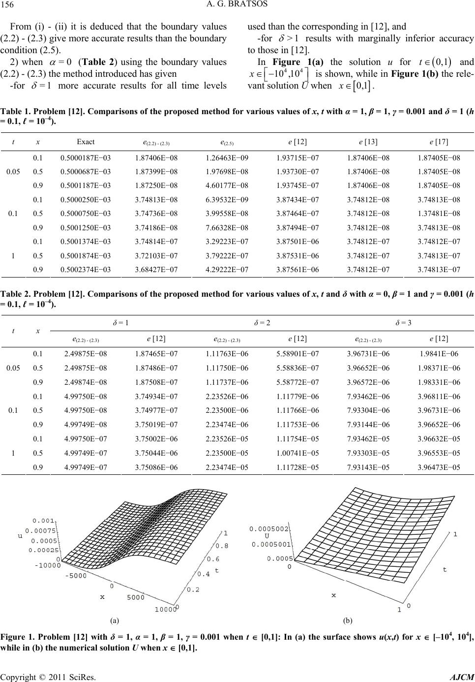 A. G. BRATSOS Copyright © 2011 SciRes. AJCM 156 From (i) - (ii) it is deduced that the boundary values (2.2) - (2.3) give more accurate results than the boundary condition (2.5). 2) when =0 (Table 2) using the boundary values (2.2) - (2.3) the method introduced has given -for =1 more accurate results for all time levels used than the corresponding in [12], and -for >1 results with marginally inferior accuracy to those in [12]. In Figure 1(a) the solution u for 0,1t and 44 10 ,10x is shown, while in Figure 1(b) the rele- vant solution U when 0,1x. Table 1. Problem [12]. Comparisons of the proposed method for various values of x, t with α = 1, β = 1, γ = 0.001 and δ = 1 (h = 0.1, ℓ = 10–4). t x Exact e(2.2) - (2.3) e(2.5) e [12] e [13] e [17] 0.1 0.5000187E−03 1.87406E−08 1.26463E−09 1.93715E−07 1.87406E−08 1.87405E−08 0.5 0.5000687E−03 1.87399E−08 1.97698E−08 1.93730E−07 1.87406E−08 1.87405E−08 0.05 0.9 0.5001187E−03 1.87250E−08 4.60177E−08 1.93745E−07 1.87406E−08 1.87405E−08 0.1 0.5000250E−03 3.74813E−08 6.39532E−09 3.87434E−07 3.74812E−08 3.74813E−08 0.5 0.5000750E−03 3.74736E−08 3.99558E−08 3.87464E−07 3.74812E−08 1.37481E−08 0.1 0.9 0.5001250E−03 3.74186E−08 7.66328E−08 3.87494E−07 3.74812E−08 3.74813E−08 0.1 0.5001374E−03 3.74814E−07 3.29223E−07 3.87501E−06 3.74812E−07 3.74812E−07 0.5 0.5001874E−03 3.72103E−07 3.79222E−07 3.87531E−06 3.74812E−07 3.74813E−07 1 0.9 0.5002374E−03 3.68427E−07 4.29222E−07 3.87561E−06 3.74812E−07 3.74813E−07 Table 2. Problem [12]. Comparisons of the proposed method for various values of x, t and δ with α = 0, β = 1 and γ = 0.001 (h = 0.1, ℓ = 10–4). δ = 1 δ = 2 δ = 3 t x e(2.2) - (2.3) e [12] e (2.2) - (2.3) e [12] e (2.2) - (2.3) e [12] 0.1 2.49875E−08 1.87465E−07 1.11763E−06 5.58901E−07 3.96731E−06 1.9841E−06 0.5 2.49875E−08 1.87486E−07 1.11750E−06 5.58836E−07 3.96652E−06 1.98371E−06 0.05 0.9 2.49874E−08 1.87508E−07 1.11737E−06 5.58772E−07 3.96572E−06 1.98331E−06 0.1 4.99750E−08 3.74934E−07 2.23526E−06 1.11779E−06 7.93462E−06 3.96811E−06 0.5 4.99750E−08 3.74977E−07 2.23500E−06 1.11766E−06 7.93304E−06 3.96731E−06 0.1 0.9 4.99749E−08 3.75019E−07 2.23474E−06 1.11753E−06 7.93144E−06 3.96652E−06 0.1 4.99750E−07 3.75002E−06 2.23526E−05 1.11754E−05 7.93462E−05 3.96632E−05 0.5 4.99749E−07 3.75044E−06 2.23500E−05 1.00741E−05 7.93303E−05 3.96553E−05 1 0.9 4.99749E−07 3.75086E−06 2.23474E−05 1.11728E−05 7.93143E−05 3.96473E−05 (a) (b) Figure 1. Problem [12] with δ = 1, α = 1, β = 1, γ = 0.001 when t [0,1]: In (a) the surface shows u(x,t) for x [–104, 104], while in (b) the numerical solution U whe n x [0,1].  A. G. BRATSOS 157 Table 3. Problem [17]. Comparisons of the proposed method for various values of δ and γ when α = β = 1 (h = 0.1, ℓ = 10–4). t = 1 δ = 1 γ = 10–3 t = 0.5 δ = 2 γ = 10–2 t = 0.5 δ = 4 γ = 10–2 x e(2.2) - (2.3) e [17] x e(2.2) - (2.3) e [17] x e(2.2) - (2.3) e [17] 0.1 3.74814E−07 3.74812E−07 0.1 3.89463E−05 2.75734E−04 0.1 5.69322E−05 1.08762E−03 0.5 3.72103E−07 3.74814E−07 0.3 3.89656E−05 2.75614E−04 0.3 5.69778E−05 1.08644E−03 0.9 3.68427E−07 3.74813E−07 0.5 3.89844E−05 2.75493E−04 0.5 5.70134E−05 1.08527E−03 Table 4. Problem [16]. Boundary conditions (2.4 ) – (2.5). Comparisons of the propose d method for various values of t withα = 5 and δ = 1 (h = 0.1, ℓ = 10–4). γ = 10–3 γ = 10–4 γ = 10–5 t β Method e [16] Method e [16] e e [16] 1 3.1570E−08 3.1616E−08 3.1584E−10 3.1630E−10 3.3410E−12 3.1632E−12 10 3.9684E−07 3.9742E−07 3.9702E−09 3.9760E−09 3.9704E−11 3.9762E−11 0.3 100 5.0291E−06 5.0365E−06 5.0316E−08 5.0389E−08 5.0318E−10 5.0392E−10 1 3.3393E−08 3.3394E−08 3.3408E−10 3.3409E−10 3.3410E−12 3.3411E−12 10 4.1976E−07 4.1977E−07 4.1995E−09 4.1996E−09 4.1997E−11 4.1998E−11 0.9 100 5.3165E−06 5.3166E−06 5.3221E−08 5.3223E−08 5.3224E−10 5.3225E−10 3.2. Problem [17] From Table 3 it is deduced that the method introduced using the boundary values (2.2) - (2.3) has given more accurate results for all time levels and parameters used than the relevant method in [17]. 3.3. Problem [16] For reasons of comparison with the relevant results in [18] the boundary conditions (2.4) - (2.5) with 0= t and 0,ut 1=1, tut were used. From Table 4 it is deduced that the proposed method: -has given marginally more accurate results to those in [16] for all time levels and , used, -for fixed , and ● , the accuracy increases and U tends to identify with u at long time level as is refined, ● , as increases, the accuracy decreases. 4. Conclusions An implicit finite difference scheme based on fourth- order rational approximants to the matrix exponential term was proposed for the numerical solution of the Bur- gers-Huxley equation. The resulting nonlinear scheme was solved using an improved predictor-corrector method. The computational efficiency of the proposed method given in detail in Section 3 was tested by comparing the numerical results to selected ones in [12,13,16,17] using both appropriate boundary values and conditions. Con- clusions for the boundaries used were derived. Since the real world problems lead to the numerical solution of nonlinear equations or systems of equations, the introduced low cost and easy-to-handle method en- ables us to obtain accurate solutions. 5. References [1] A. L. Hodgkin and A. F. Huxley, “A Quantitative De- scription of Ion Currents and Its Applications to Conduc- tion and Excitation in Nerve Membranes,” Journal of Physiology, Vol. 117, No. 4, 1952, pp. 500-544. [2] J. Satsuma, “Topics in Soliton Theory and Exactly Solv- able Nonlinear Equations,” In: M. Ablowitz, B. Fuch- ssteiner and M. Kruskal, Eds., World Scientific, Singa- pore City, 1987. [3] X. Wang, “Nerve Propagation and Wall in Liquid Crys- tals,” Physics Letters, Vol. 112A, No. 8, 1985, pp. 402-406. [4] X. Y. Wang, Z. S. Zhu and Y. K. Lu, “Solitary Wave Solutions of the Generalised Burgers-Huxley Equation,” Journal of Physics A: Mathematical and General, Vol. 23, No. 3, 1990, pp. 271-274. doi:10.1088/0305-4470/23/3/011 [5] A. G. Bratsos, “A Fourth-Order Numerical Scheme for Solving the Modified Burgers Equation,” Computers and Mathematics with Applications, Vol. 60, No. 5, 2010, pp. 1393-1400. doi:10.1016/j.camwa.2010.06.021 [6] R. Fitzhugh, “Mathematical Models of Excitation and Propagation in Nerve,” In: H. P. Schwan. Ed., Biological Engineering, McGraw Hill, New York, 1969, pp. 1-85. [7] P. G. Estévez and P. R. Gordoa, “Painlevé Analysis of the generalized Burgers-Huxley Equation,” Journal of Phys- ics A: Mathematical and General, Vol. 23, No. 21, 1990, Copyright © 2011 SciRes. AJCM  158 A. G. BRATSOS pp. 4831-4837. [8] P. G. Estévez, “Non-Classical Symmetries and the Sin- gular Manifold Method: The Burgers and the Bur- gers-Huxley Equations,” Journal of Physics A: Mathe- matical and General, Vol. 27, No. 6, 1994, pp. 2113- 2127. [9] O. Yu. Yefimova and N. A. Kudryashov, “Exact Solu- tions of the Burgers-Huxley Equation,” Journal of Ap- plied Mathematics and Mechanics, Vol. 68, No. 3, 2004, pp. 413-420. doi:10.1016/S0021-8928(04)00055-3 [10] X. Deng, “Travelling Wave Solutions for the Generalized Burgers-Huxley Equation,” Applied Mathematics and Computation, Vol. 204, No. 1, 2008, pp. 733-737. doi:10.1016/j.amc.2008.07.020 [11] A. M. Wazwaz, “Analytic Study on Burgers, Fisher, Huxley Equations and Combined Forms of These Equa- tions,” Applied Mathematics and Computation, Vol. 195, No. 2, 2008, pp. 754-761. doi:10.1016/j.amc.2007.05.020 [12] H. N. A. Ismail, K. Raslan and A. A. A. Rabboh, “Adomian Decomposition Method for Burger’s Huxley and Burger’s-Fisher Equations,” Applied Mathematics and Computation, Vol. 159, No. 1, 2004, pp. 291-301. doi:10.1016/j.amc.2003.10.050 [13] I. Hashim, M. S. M. Noorani and M. R. S. Al-Hadidi, “Solving the Generalized Burgers-Huxley Equation Us- ing the Adomian Decomposition Method,” Mathematical and Computer Modelling, Vol. 43, No. 11-12, 2006, pp. 1404-1411. doi:10.1016/j.mcm.2005.08.017 [14] M. Javidi, “A Numerical Solution of the Generalized Burger’s-Huxley Equation by Pseudospectral Method and Darvishi’s Preconditioning,” Applied Mathematics and Computation, Vol. 175, No. 1, 2006, pp. 1619-1628. doi:10.1016/j.amc.2005.09.009 [15] M. Javidi, “A Numerical Solution of the Generalized Burgers-Huxley Equation by Spectral Collocation Method,” Applied Mathematics and Computation, Vol. 178, No. 2, 2006, pp. 338-344. [16] M. Javidi and A. Golbabai, “A New Domain Decomposi- tion Algorithm for Generalized Burgers-Huxley Equation Based on Chebyshev Polynomials and Preconditioning,” Chaos Soliton & Fractals, Vol. 39, 2009, pp. 849-857. [17] B. Batiha, M. S. M. Noorani and I. Hashim, “Application of Variational Iteration Method to the Generalized Bur- gers-Huxley Equation,” Chaos Solitons & Fractals, Vol. 36, No. 3, 2008, pp. 660-663. doi:10.1016/j.chaos.2006.06.080 [18] A. Khattak, “A Computational Meshless Method for the Generalized Burgers-Huxley Equation,” Applied Mathe- matical Modelling, Vol. 33, No. 9, 2009, pp. 3718-3729. doi:10.1016/j.apm.2008.12.010 [19] E. Babolian and J. Saeidian, “Analytic Approximate So- lutions to Burgers, Fisher, Huxley Equations and Two Combined Forms of These Equations,” Communications in Nonlinear Science and Numerical Simulation, Vol. 14, 2009, pp. 1984-1992. doi:10.1016/j.cnsns.2008.07.019 [20] B. Fornberg, “A Practical Guide to Pseudospectral Meth- ods,” Cambridge University Press, Cambridge, 1998. [21] E. H. Twizell, “Computational Methods for Partial Dif- ferential Equations,” Ellis Horwood Limited, Chichester, 1984. Copyright © 2011 SciRes. AJCM
|