Journal of Electromagnetic Analysis and Applications
Vol.4 No.6(2012), Article ID:20341,2 pages DOI:10.4236/jemaa.2012.46037
Revisiting Magnetic Net and a Bouncing Magnetic Ball
![]()
Department of Physics, Pennsylvania State University, York, USA.
Email: has2@psu.edu
Received April 24th, 2012; revised May 20th, 2012; accepted May 28th, 2012
Keywords: Magnetic Net; Induced Current; Mathematica
ABSTRACT
Recently the author reported the feasibility of envisioning a scenario where a massive permanent magnetic dipole bounces off and oscillates about an invisible horizontal magnetic net in the presence of gravity. The scenario has been revisited, modifying its physical contents. The modification embodies analysis of the impact of the induced current due to the falling magnetic dipole. The induced current counteracts the conduction current and alters the dynamics and kinematics of the motion. This rapid communication reports the recent advances.
1. Motivations and Goals
In [1] we utilize the well-known recipe for a magnetic field of a looping conduction DC along the symmetry axis perpendicular to the plane of the loop. The inhomogeneity of the field along this axis causes the field to exert an attractive force on a permanent magnetic dipole with its magnetic moment aligned with the field. In a scenario where the symmetry axis is vertical and so gravity is present we justified the feasibility of oscillations of a loose permanent magnet. Interested readers may review [1] for details.
We revisit the given scenario outlined above modifying its physical content by including the induced current due to the rate of change of magnetic flux of the falling magnet through the loop. For the sake of simplicity we assume this change comes about from the variation of the axial component of the magnetic field of the magnetic dipole. This puts the characteristics of these two fields, the field of the conduction current and the field of the magnetic dipole in the same footing. The character of the azimuthal field is addressed in [2].
Magnetic field of the DC looping current along the symmetry axis of the loop is,
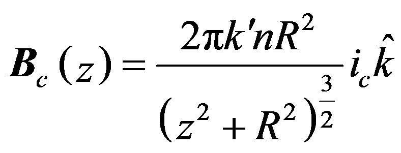 (1)
(1)
where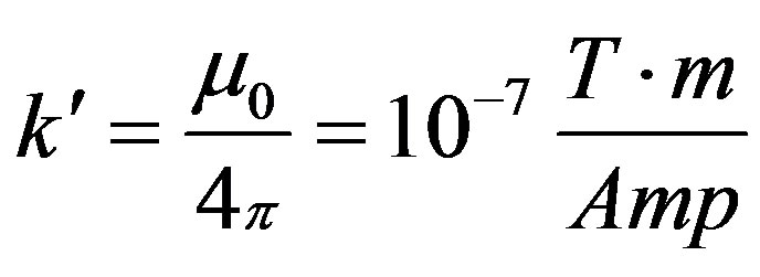 , R, n and ic are the radius of the loop, number of the turns and the conduction current, respectively.
This yields the magnitude of the magnetic force,
 (2)
(2)
where µ is the magnetic moment of the permanent magnet. Equation (1) with a few modifications is written as,
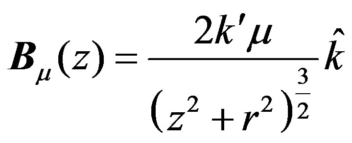 (3)
(3)
This equation is to apply to a cylindrical permanent magnetic dipole of a circular base radius r and a magnetic dipole moment µ. The flux of this field through the area of the circular looping DC is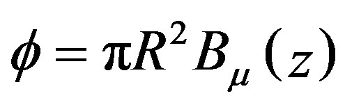 . Its rate of change is the induced emf conducive the induced current, iind. Combining these pieces yields,
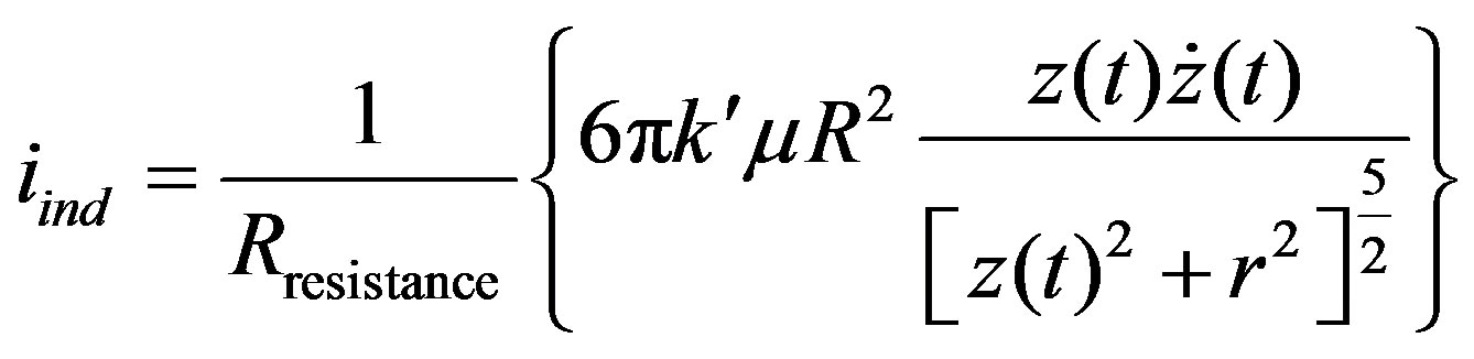 (4)
(4)
where Rresistance is the ohmic resistance of the conduction loops.
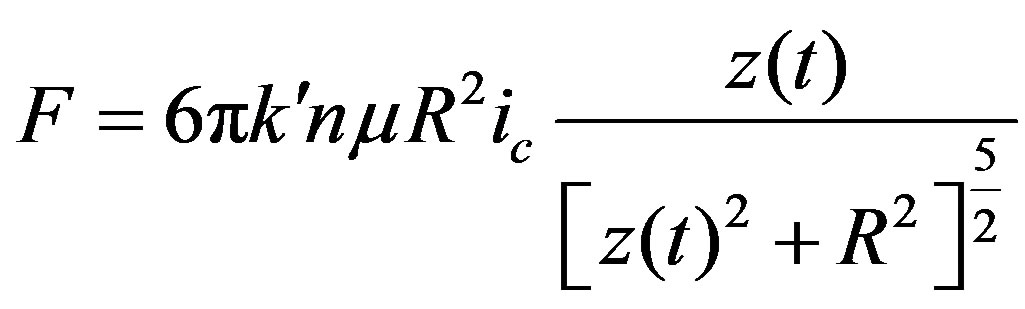
The induction current given by Equation (4) counteracts the conduction current, ic modifying the force F given by Equation (2) to its effective value,
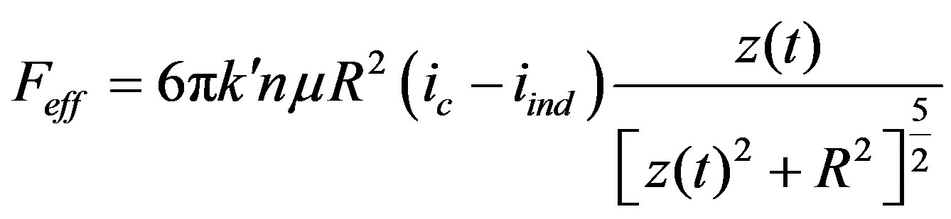 (5)
(5)
Utilizing Feff the equation of motion for the permanent magnet of mass m becomes,
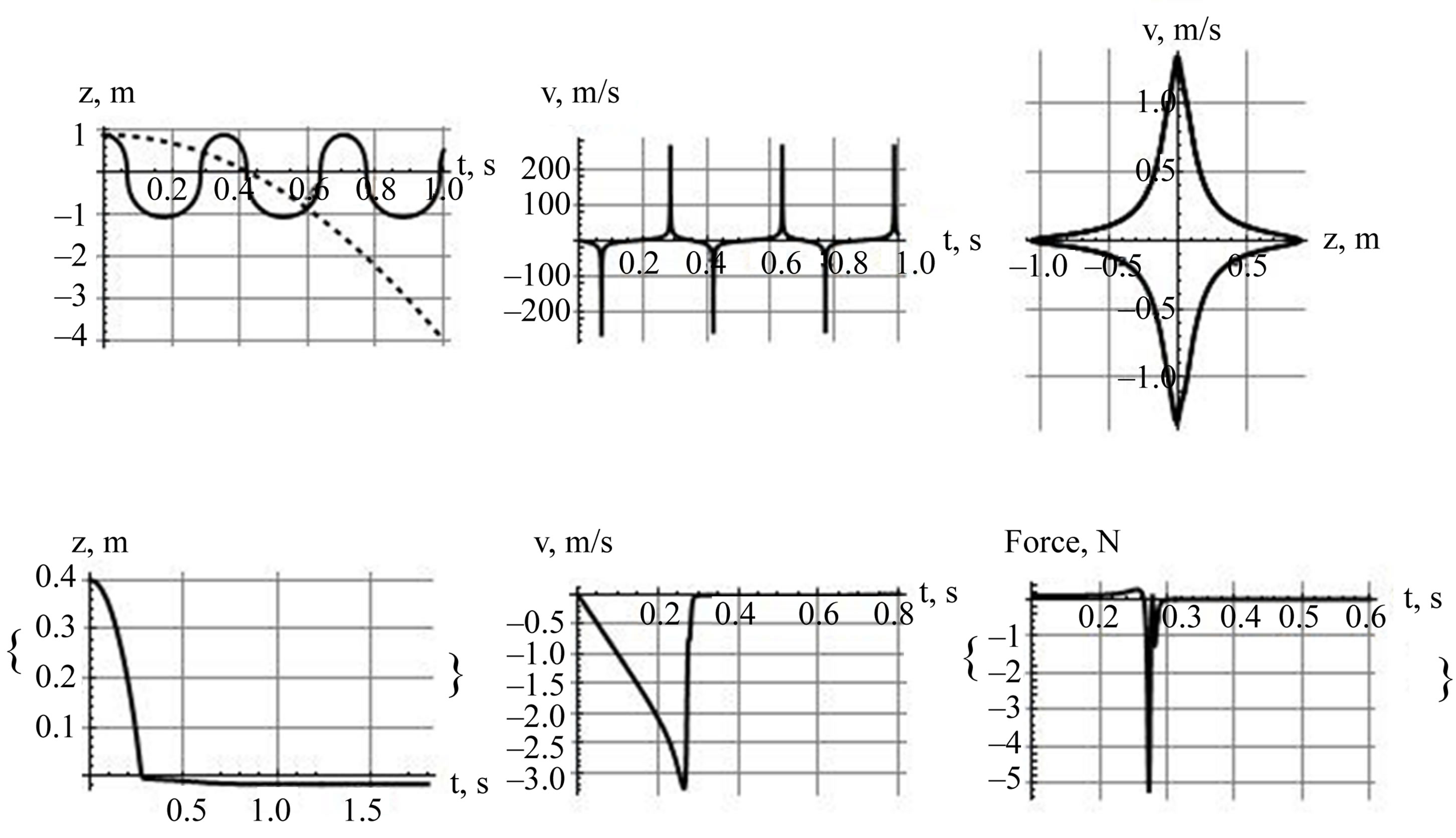
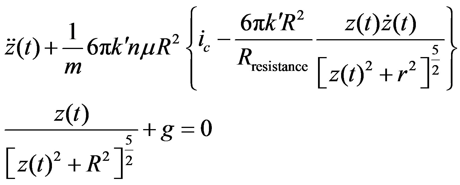
Figure 1. The top row are the graphs reported in [1]. The first two graphs of the second row are their equivalents utilizing parameters compiled in values. The third graph of the second row is the corresponding active force.
 (6)
(6)
At first glance one realizes the order of magnitude of the second term in the brace is O(k'2). Knowing the k' is small, one concludes the impact of the iind when compared to ic is negligible. Therefore, the dynamics of the falling magnet is being controlled solely by the conduction current. In fact implicitly we have utilized Feff = F in [1]. However, if one considers resistances as small as mΩ range this changes the scenario considerably. For instance with the parameters stored in values in MKS units utilizing Mathematica [3] we solve Equation (6) numerically. What follows are the graphic display of the results.
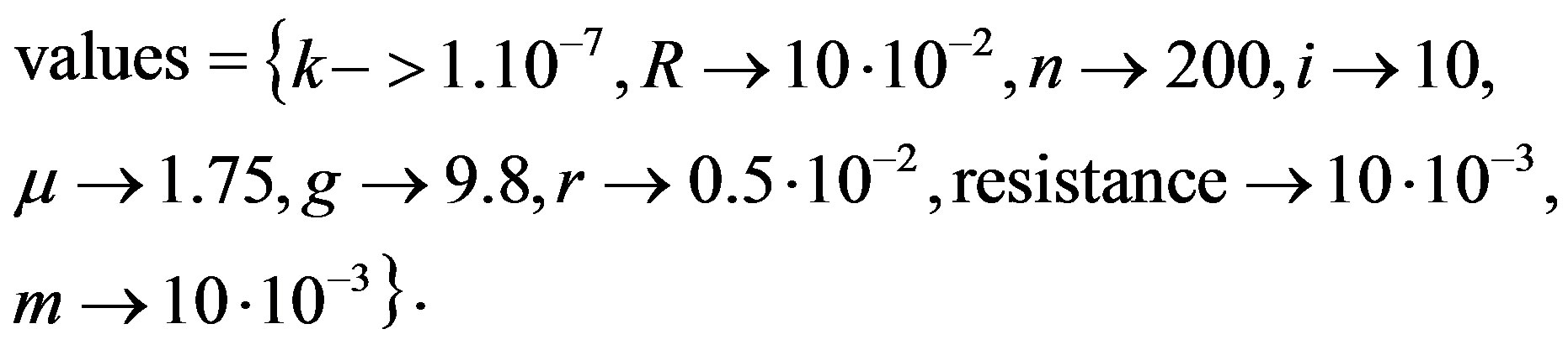
As shown in the first row of Figure 1, for chosen parameters in [1] a freely dropped magnetic dipole oscillates about the magnetic net. The dashed line is added and serves as a reference; it is the position of the free falling magnet from the loop. The phase diagram, the third graph, is the signature character of an oscillator. In our current analysis with the parameters stored in values the impact of the induced current is shown in the plots of the second row. Accordingly, the induced current softens the attractive magnetic DC force. The profile of the active force vs. time is depicted in the last graph of the second row. The magnet after a few irregular oscillations comes to a halt and settles underneath the loop. In other words, the induced current dampens the motion, preventing the magnet to oscillate steady. At the final resting position the induced current is inactive, and the DC driven attractive magnetic force equalizes the gravity. Interested readers may consider a different set of range parameters for the resistance and the mass conducive to various scenarios.
2. Conclusion
The author analyzes the impact of the induced current on the equation of motion of a mobile permanent magnetic dipole in the presence of an inhomogeneous magnetic field of a DC. It is shown that by selecting a set of thoughtful parameters the value of the induced current effectively may interfere with the conduction current resulting in curious outcomes.
REFERENCES
- H. Sarafian, “Magnetic Net and a Bouncing Magnetic Ball,” Springer-Verlag, Berlin, 2012.
- H. Sarafian, “Symbolic Computation and Graphic Presentation of Magneto-static Field and its Associated Vector Potential,” Journal of Electromagnetic Analysis and Applications, Vol. 3, No. 5, 2011, pp. 172-177. doi:10.4236/jemaa.2011.35028
- Mathematica V 8.01, Wolfram Research Inc., Champaign.