Journal of Electromagnetic Analysis and Applications
Vol. 2 No. 5 (2010) , Article ID: 1920 , 9 pages DOI:10.4236/jemaa.2010.25042
Generalized Alternating-Direction Implicit Finite-Difference Time-Domain Method in Curvilinear Coordinate System*
![]()
1Center for Electromagnetic Simulation, School of Information Science and Technology, Beijing Institute of Technology, Beijing, China; 2Department of Electronic Engineering, Queen Mary, University of London, London, United Kingdom.
Email: wsong@bit.edu.cn, yang.hao@elec.qmul.ac.uk
Received February 1st, 2010; revised March 26th, 2010; accepted April 3rd, 2010.
Keywords: Alternating Direction Implicit technique, numerical instability, nonorthogonal FDTD
ABSTRACT
In this paper, a novel approach is introduced towards an efficient Finite-Difference Time-Domain (FDTD) algorithm by incorporating the Alternating Direction Implicit (ADI) technique to the Nonorthogonal FDTD (NFDTD) method. This scheme can be regarded as an extension of the conventional ADI-FDTD scheme into a generalized curvilinear coordinate system. The improvement on accuracy and the numerical efficiency of the ADI-NFDTD over the conventional nonorthogonal and the ADI-FDTD algorithms is carried out by numerical experiments. The application in the modelling of the Electromagnetic Bandgap (EBG) structure has further demonstrated the advantage of the proposed method.
1. Introduction
The Finite-Difference Time-Domain (FDTD) Method [1] has been proven to be an effective algorithm in computational electromagnetics. The first FDTD algorithm was introduced by Yee [2] in 1966. Since then, extensions of this method [3-8] have been made continuously. The nonorthogonal FDTD (NFDTD) method [9-11] is a standard generalized FDTD algorithm based on the curvilinear coordinate system. As far as a curved geometry is concerned, the NFDTD algorithm has demonstrated improved efficiency over the conventional Yee’s algorithm [12], due to the fact that considerably fewer cells are needed in the former by using conformal meshes instead of employing staircase approximation.
As is the case in the Cartesian FDTD algorithm, the time interval dtmax used in the NFDTD method is constrained by the Courant-Friedrich-Levy (CFL) stability condition [13]. Consider a two-dimensional NFDTD cell shown in Figure 1, ξi and ηj denote the skewed coordinates, and θij (i and j are cell indices) denotes the rotating angle from ξi to ηj. The Courant criterion for this particular cell (i, j) is donated as dtmaxi,j. The time increment dt used in the NFDTD simulation should not exceed the Courant criterion dtmax given by (1), which is the minimum value of dtmaxi,j, in order to guarantee that the CFL condition is satisfied for every cell in the NFDTD meshes. The orthogonal CFL condition is a special case when θ = 90º.
For orthogonal meshes, it is straightforward to calculate dtmax. However, with nonorthogonal meshes, it is not trivial to find the minimum value of dtmaxi,j as diverse cells exist. More to the point, when the meshes contain globally large but locally very small or skewed cells, the using of the smallest dtmaxi,j may result in low efficiency in the NFDTD simulations.
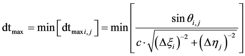 (1)
(1)
In addition, it has been proven that the NFDTD approach suffers late-time numerical instabilities [13-15]. Various efforts have been made to alleviate this problem [16- 18].
The alternating direction implicit (ADI) technique has been successfully applied to the orthogonal FDTD instead of the Yee’s leapfrogging scheme, resulting in the
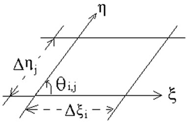
Figure 1. A two-dimensional nonorthogonal FDTD cell
removal of the CFL stability condition and an improvement in the efficiency of FDTD method. In [19], the ADI principle as applied in [6] and [7] is extended to the curvilinear coordinates based on Lee’s NFDTD scheme and a novel NFDTD method that is free of the CFL stability condition is briefly introduced. Similar idea was proposed based on Holland’s NFDTD formulation in [20]. In this paper, the formulation of the generalized ADINFDTD as in [19] is presented in details and its numerical efficiency and accuracy is further studied. Compared to the conventional NFDTD method, the numerical efficiency can be improved by using an increased dt, and the late time instability of the NFDTD scheme has been greatly reduced. Compared with the conventional orthogonal ADI-FDTD, this generalized scheme is not unconditionally stable. However, it shows improved numerical efficiency in modelling curved structures by requiring less computer memory and computer run time, because coarser conformal grids are employed. In order to demonstrate its efficiency, the proposed ADI-NFDTD is applied in calculating the bandgap diagram of the Electromagnetic Bandgap structure (EBGs).
2. Formulation
The Maxwell curl equations can be written as the following for a source-free space:
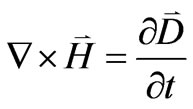 (2)
(2)
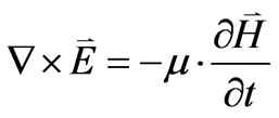 (3)
(3)
where μ is the medium permeability. Both of the equations can be casted into partial differential equations in the curvilinear coordinates as shown in [15]. A 2-D TE wave module is used to illustrate the scheme. The formulation for the TM module can be obtained in a similar way.
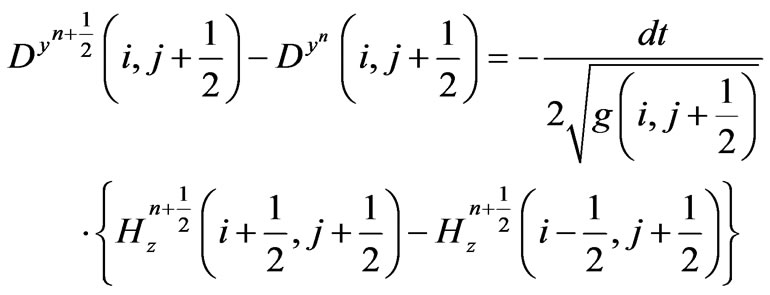
Two procedures are used to solve the differential equations. The first procedure is based on (4)-(6), and the second procedure is based on (7)-(9).
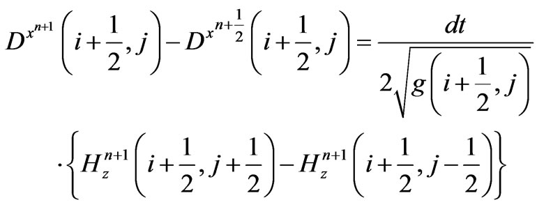
1) The First Procedure:
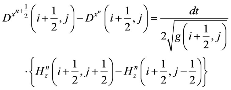 (4)
(4)
 (5)
(5)
 (6)
(6)
2) The Second Procedure:
 (7)
(7)
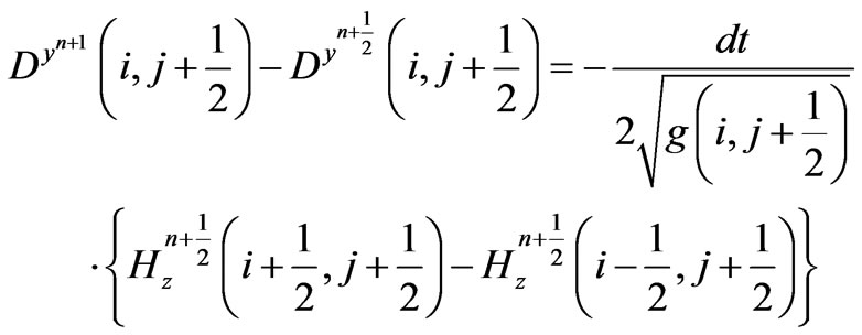 (8)
(8)
 (9)
(9)
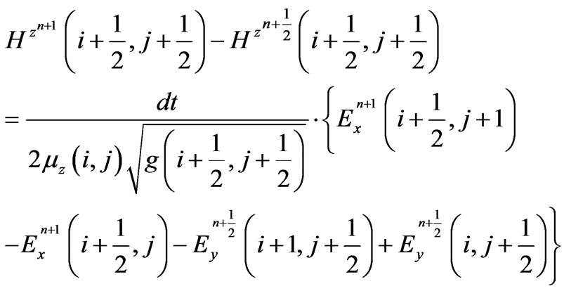
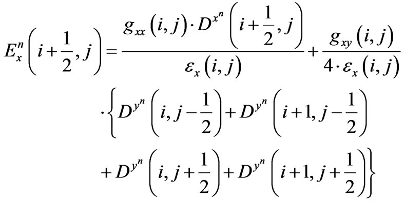
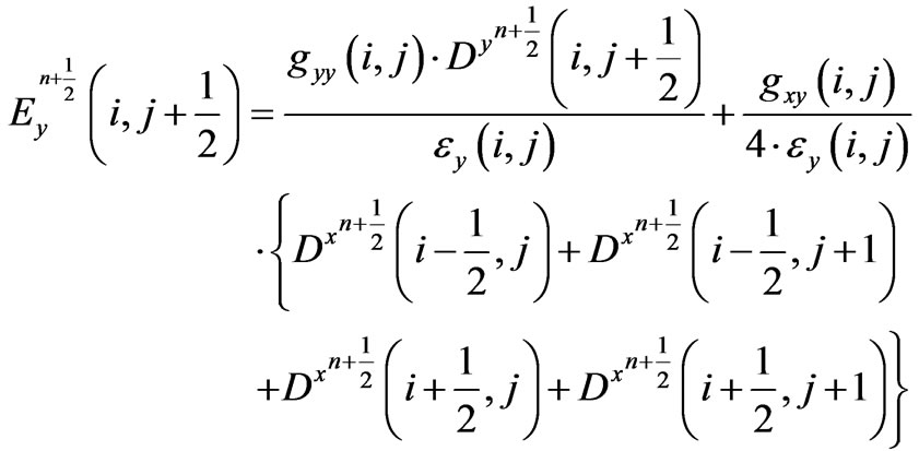
where Ex, Ey, Hz are the covariant electric and magnetic field components which represent the flow of field along the grid, while Dx, Dy and Hz are the contravariant electric fluxes and magnetic field component which represent the flow going through the facets of the grid. μz is the medium permeability for calculating Hz and g is the metric tensor computed from the local curvilinear coordinates. The covariant field components (Ex and Ey) must be calculated from the contravariant flux (Dx and Dy) by interpolating equations as introduced in the conventional NFDTD scheme [9-10]. As the covariant field components should be valued in the same position with their contravariant pairs, the neighbouring averaging projection scheme is employed. For a 2-D model, gxz and gyz are zeros, and gzz equals to unity for every cell. Hence we obtain (10)-(14).
 (10)
(10)
 (11)
(11)
 (12)
(12)
 (13)
(13)
 (14)
(14)
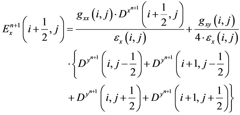
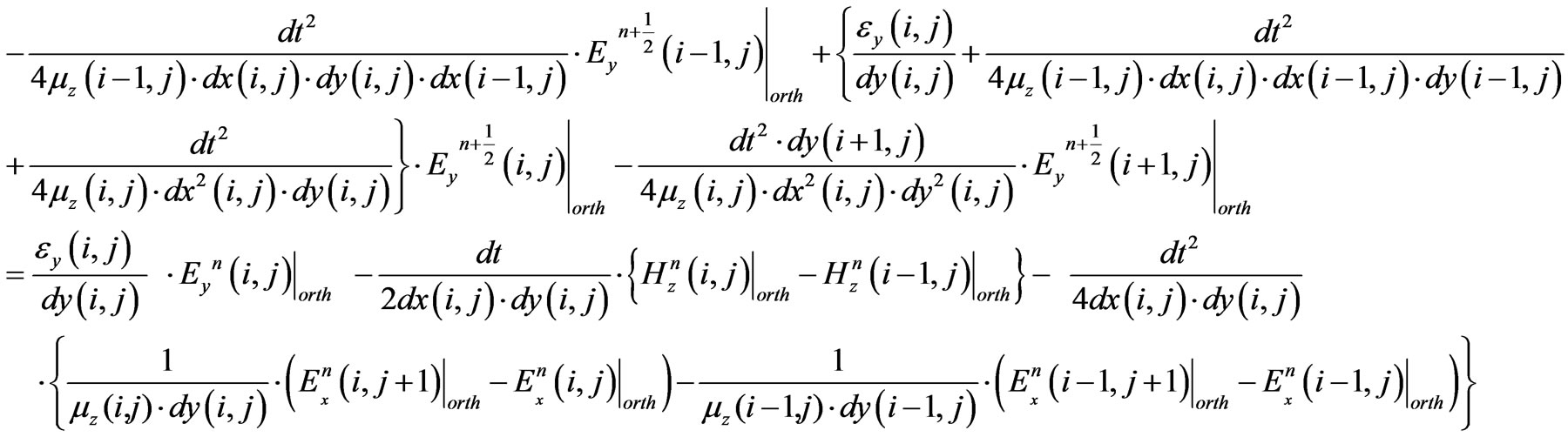
where εi (i = x, y) is the material permittivity in the xor ydirection. By substituting (10), (11) and (13) into (6) and the resulting expression for  into (5), one can obtain (15). From (15) the cell indices (i,j) are used in the equations for a neat presentation, e.g.,
  is used instead of
 . With
  readily obtained by (4), (15) is a tri-diagonal system of equation that can be easily solved.
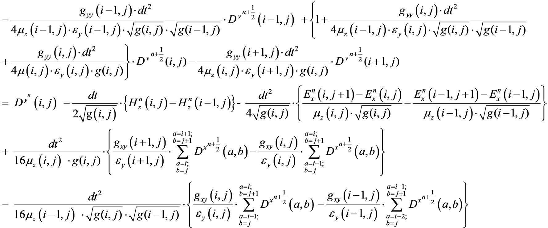 (15)
(15) Thus  is updated. Then
  can be calculated by (6).
The field components in the second procedure can be updated in a similar way, by the use of (11), (12), (14) and (7)-(9).
The proposed ADI-NFDTD algorithm is an extension of the ADI-FDTD in the curvilinear coordinate system. As a result, if the grid is uniform and orthogonal, this algorithm will reduce to the conventional orthogonal ADI-FDTD, as illustrated in (16)-(21).
We apply the following relations to the derived ADINFDTD equations:
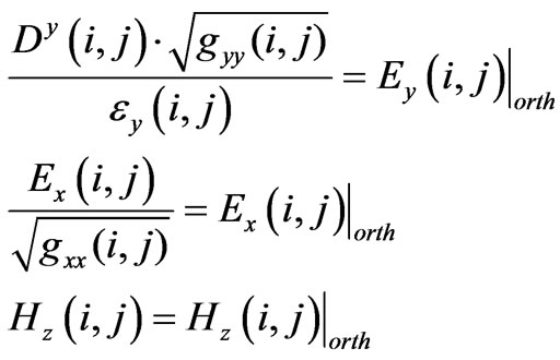 (16)
(16)
where 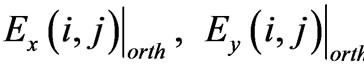 and
and  denote
the corresponding electric and magnetic field components in the Cartesian coordinates respectively.
The g tensors have the relationship of (17) under 2-D orthogonal meshes.
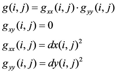 (17)
(17)
Substituting (16)-(17) into (15) yields (18), which is the ADI-FDTD updating equation under arbitrary orthogonal meshes.
 (18)
(18) Given that the FDTD grid is uniform, and denoting the spatial increments along the xand yaxes as Δx and Δy, respectively, (19) are yielded from (17).
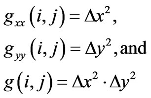 (19)
(19)
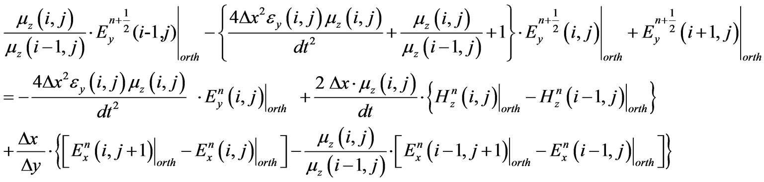 (20)
(20)
Then substituting (19) into (18) and multiplying  on both side of the equation yields (20). Equation (20) is the general equation for orthogonal ADI-FDTD scheme with uniform grid. Equations (18) and (20) can treat homogeneous or inhomogeneous, isotropic or anisotropic media. In a medium where μz (i, j) = μz (i-1, j), (20) further reduces to the formula given in [6].
3. Numerical Results
3.1 Comparison of the Late Time Instability and the Numerical Accuracy of the ADI-NFDTD Algorithm with the Conventional NFDTD Algorithm
The resonant modes of a cylindrical perfect electric conductor (PEC) cavity resonator are calculated by using both the conventional NFDTD and the proposed ADINFDTD schemes. The radius of the resonator is 0.15m and the structure is infinitely long. The cavity is filled with vacuum of permittivity εr = 1. The outer material is PEC, and the whole computational region is 0.56 m × 0.56 m meshed by 25 × 26 cells. A sine modulated cosine pulse (21) is excited inside the cavity to provide a wide band excitation to excite all the possible TE modes:
 (21)
(21)
where Am relates to the amplitude of the signal, f is the frequency parameter, dt is the time increment and n is the iteration index.
The temporal signatures of the magnetic fields inside the resonator are recorded. The first 8,000 time steps results from both the conventional and the ADINFDTD algorithms are normalized by their own peak values and are plotted in Figure 2.
More simulations were performed using different dt values to study the stability and the accuracy of the ADINFDTD scheme. It is shown that unlike the conventional
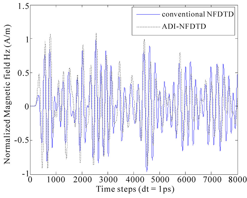
Figure 2. The normalized H field results of the first 8000 time steps from the two schemes
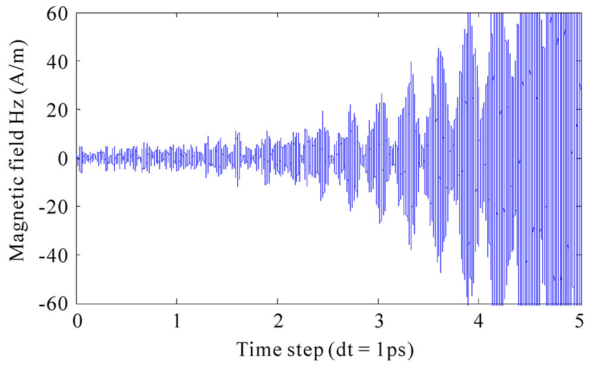
ADI-FDTD, this generalized ADI-NFDTD scheme is not an unconditionally stable scheme. Instability in the temporal results is observed when small dt (i.e., comparable with or smaller than the dtmax required in the NFDTD scheme) is used. However, compared to the NFDTD scheme, the unstable result in the ADI-NFDTD occurs much later and the spurious energy grows much slower than that in the conventional NFDTD scheme. This is demonstrated in Figure 3.
The removal of the CFL stability condition on dt in the ADI-NFDTD method is also observed. When dt reaches 16ps in the simulations, the conventional NFDTD cannot provide reasonable results, indicating that the CFL stability condition is violated, while ADI-NFDTD scheme can do so, even using a greater dt value.
In order to compare the accuracy of the ADI-NFDTD with the conventional NFDTD algorithm, the resonant frequencies are calculated using the Fast Fourier Transformation (FFT) and are compared with the analytical results. Since both the NFDTD and the ADI-NFDTD methods suffer numerical instability in late time steps, the temporal data are truncated to 40,000 and 100,000 time steps respectively. Such numbers are chosen in order to obtain the best frequency resolutions, and avoid too much spurious energy in the spectra at the same time. Since dt = 1 ps, the frequency resolutions of the conventional and the ADI-NFDTD results are 0.025 GHz and 0.01 GHz respectively. The calculated resonant frequency spectra are plotted in Figure 4.
As can be seen, it is possible to distinguish two closelyspaced frequency spectra from the results obtained by using the ADI-NFDTD, while it is hard to do so in the conventional NFDTD due to the limited frequency resolution. Moreover, the noise level of the ADI-NFDTD is lower than that of the conventional NFDTD, if dt used in the two simulations are comparable.
 (a)
(a)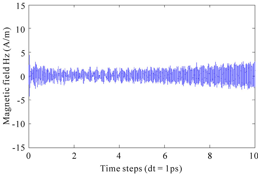 (b)
(b)
Figure 3. Hz field temporal results of (a) the conventional NFDTD scheme, and (b) the ADI-NFDTD scheme, with time interval dt = 1 ps
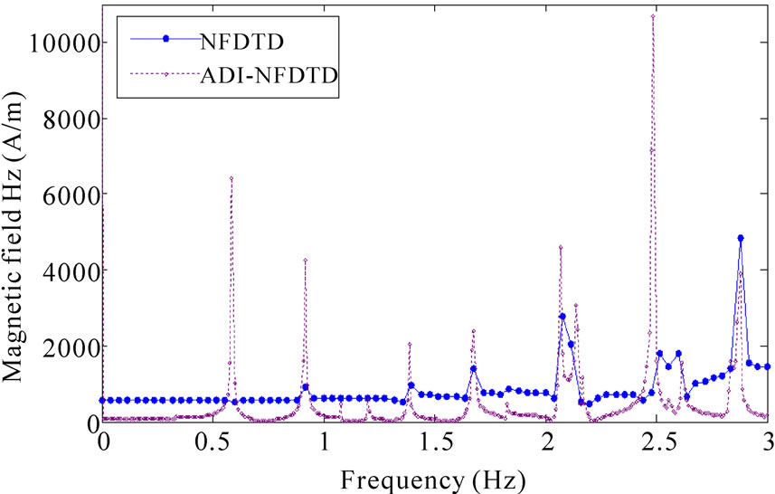
Figure 4. Resonant frequency spectra of the cavity resonator calculated from the two schemes, with dt = 1 ps. After [19]
In order to compare the accuracy of the two NFDTD schemes, the averaged relative error rate of the resonant frequency as a function of the relative time interval is introduced. This error rate is calculated in the following manner. Firstly, the absolute value of the difference of the calculated resonant frequency with the theoretical one is divided by the latter, and expressed in percentage, forming the relative error rate for each resonant mode. Then, the standard deviation of the relative error rates of all the modes within frequency band of interest (0-3 GHz) are calculated as the averaged relative error rate of the numerical results. The curve of the averaged relative error rate as the function of time interval is plotted in Figure 5.
In theory, the ADI-NFDTD may not necessarily provide better accuracy than the conventional NFDTD. However, to the best of the authors’ knowledge, the former can always provide more stable temporal results than the latter. As the FFT being performed with a sufficient frequency resolution, the ADI-NFDTD shows smaller relative error rate at some dt values in Figure 5. The removal of the CFL condition on NFDTD algorithm can be seen when dt is greater than 16 ps. However, according to the authors’ simulation experience, dt should not exceed the corresponding Courant criterion dtmax in order to maintain the accuracy in ADI-NFDTD simulations. By using the same dt, the computational efficiency is decreased in the ADI-NFDTD simulation than in the NFDTD one.
3.2 Comparison of the Numerical Efficiency and Accuracy of the ADI-NFDTD Algorithm with the ADI-FDTD Algorithm
A two-dimensional cavity resonator is modelled using both the ADI-NFDTD and the conventional orthogonal ADI-FDTD algorithms, in order to demonstrate the numerical efficiency improvement of the former scheme. The radius of the cavity is 0.15 m. The cavity is filled with vacuum of relative permittivity εr = 1. The outer material is copper, with relative permittivity εr = 1 and conductivity σ = 5.8 × 10⁷ S/m. The whole computational region is 0.6 m × 0.6 m, meshed by the ADI-NFDTD method using 46 × 46 cells, and by the orthogonal ADI-FDTD method using 60 × 60, 70 × 70 and 80 × 80 cells respectively. The time step is chosen to be 2 ps and 25,000 iterations are run in each simulation. A modulated Gaussian pulse as shown in (22) is excited inside the cavity. The temporal responses of probed points inside the cavity are recorded and Fourier Transformed, after which the resonant frequencies is identified as peaks in the frequency spectra.
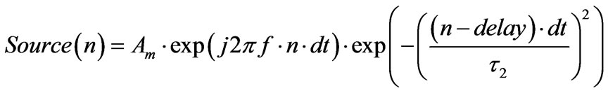 (22)
(22)
where Am is the maximum amplitude, f is the frequency parameter, n is the iteration index, dt is the time increment, 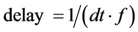 is the delay of the pulse in time step, and
 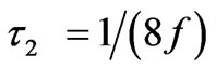 is the pulse half-duration at the 1/e point. In the simulation, Am=1 and f = 0.5 GHz.

Figure 5. The averaged relative error rate of the resonant frequency calculated by the conventional NFDTD and the proposed ADI-NFDTD schemes as the function of relative time interval dt/dt0 (dt0 = 1ps). After [19]
To calculate the relative error rates (RERs), the frequencies of all the genuine modes are compared with the theoretical results [22], and the results are shown in Table 1.
Table 2 presents a comparison of numerical errors, computer resources used in all simulations in the same computer under the same programming environment of Matlab 6. The averaged relative error rate calculated from the genuine and the spurious modes and that from only the genuine modes are denoted as ‘ARER’ and ‘ARER-G’, respectively.
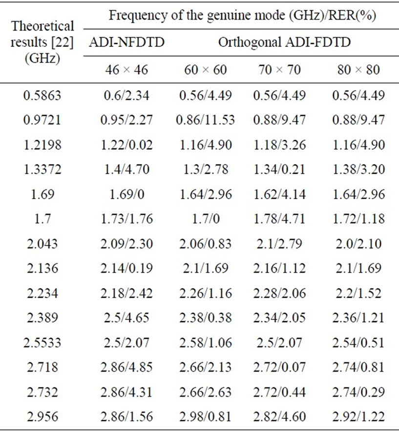
Table 1. Comparison of the numerical accuracy in terms of the genuine modes calculated by the ADI-NFDTD and orthogonal ADI-FDTD algorithms under different spatial resolutions
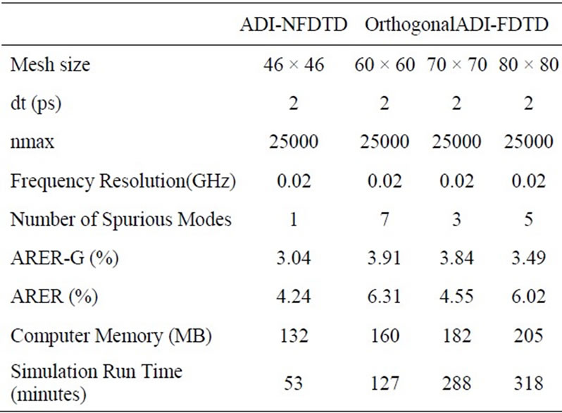
Table 2. Comparison of the accuracy and computer resources of the ADI-NFDTD and the orthogonal ADI-FDTD in calculating the resonant modes of the copper cavity
It can be seen that the ADI-NFDTD method can provide results with less numerical error while using less computer memory and less simulation run time. This demonstrates the accuracy and computing efficiency improvement of the ADI-NFDTD algorithm over the orthogonal ADI-FDTD. However, compared to the orthogonal ADI-FDTD algorithm, the ADI-NFDTD method is not an unconditionally stable method. The late time instability inherited from the NFDTD scheme is a major drawback of the ADI-NFDTD method.
3.3 Application of ADI-NFDTD Algorithm in Bandgap Structure Simulations
In this section, the ADI-NFDTD scheme is applied to model an electromagnetic bandgap (EBG) structure and the simulation results are compared with those from the NFDTD modelling.
The two-dimensional EBG structure comprises of metallic rods periodically loaded in square lattice in free space. The unit cell approach [23] is used in this model.
This EBG structure is infinite in the xand the y-direction with a lattice constant (period) a. In the z-direction, the rods are infinitely long. Each rod is made from copper with relative permittivity εr = 1 and conductivity σ = 5.8 × 10⁷ S/m. The ratio of the radius r to the lattice constant a is chosen to be r/a = 0.2. The unit cell, the Brillouin Zone and the nonorthogonal mesh file used in both the ADI-NFDTD and NFDTD algorithms are shown in Figure 6.
The dispersion diagram calculated by NFDTD is plotted in Figure 7. In the NFDTD simulation, while calculating the frequency spectra for vectors near vector k = ΓM, the time domain signals exhibit instability quickly. This will cause difficulty in obtaining the dispersion diagram. However, this problem can be easily solved by using the ADI-NFDTD algorithm.
 (a)
(a)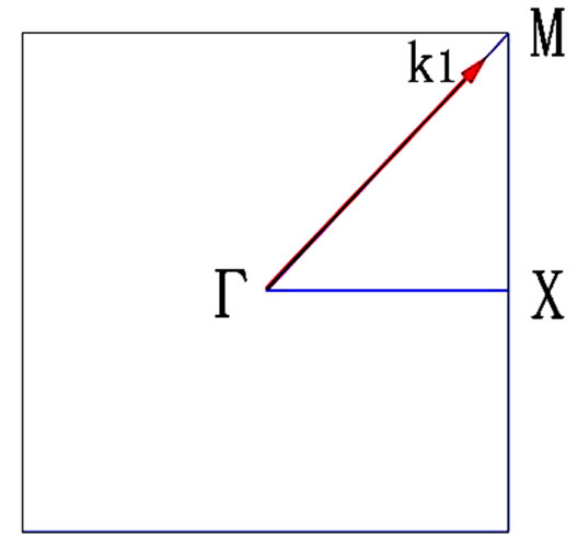 (b)
(b) (c)
(c)
Figure 6. (a) The unit cell of the EBGs; (b) the Brillouin Zone in the reciprocal lattice with k = k1 shown by a red vector; (c) the conformal mesh of the real lattice
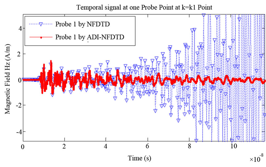
Take the eigen-mode calculation on one wave vector k = k1 (Figure 6(b)) for example. The temporal results at the same probe position obtained by using the ADINFDTD and the conventional NFDTD are compared in Figure 8. As can be seen from Figure 8(b), the ADINFDTD result shows resemblance with the NFDTD one at the beginning of simulations. It is noted that, after the first 50 nanoseconds, the results obtained via the ADI-NFDTD still remain stable while those from the NFDTD experience an exponential growth signaling numerical instability.
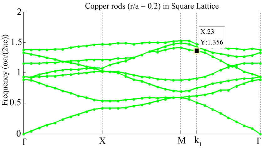
Figure 7. The dispersion diagram of the square lattice EBG, TE mode results, calculated using the NFDTD method
 (a)
(a)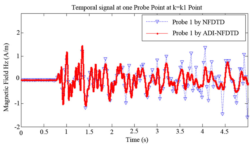 (b)
(b)
Figure 8. (a) The comparison of the temporal responses when calculating k = k1; (b) The enlarged view of the first 50 nanosecond signals of (a)
Consequently, the frequency spectra obtained using the ADI-NFDTD show a reduced noise level and hence lead to more accurate solutions for identifying eigenmodes in the dispersion diagram, as shown in Figure 9. For instance, the mode at a normalized frequency of 1.36 (highlighted using the datatip in Figure 7) can be hardly detected from the NFDTD results as the NFDTD spectrum is heavily buried by the noise. However, this mode is clearly shown as a distinct peak in the ADI-NFDTD spectra.
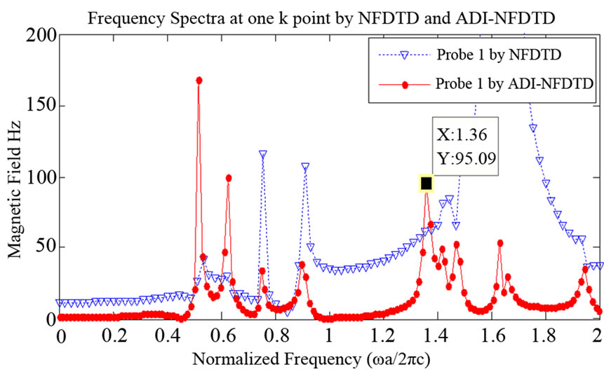
Figure 9. The comparison of the frequency spectra in calculating k = k1 using the conventional and the ADI-NFDTD algorithms
4. Conclusions
In this paper, the ADI-FDTD scheme is extended into the nonorthogonal coordinate system to achieve an ADINFDTD algorithm. The stability, accuracy and efficiency of the proposed scheme are validated by the cylindrical resonator simulations. It is shown that the CFL condition of NFDTD is removed by the use of the ADI scheme. Secondly, although the ADI-NFDTD is not unconditionally stable, the unstable result occurs at a much later stage compared with the conventional NFDTD algorithm, which is a significant improvement in terms of late time instability.
In this way, the ADI-NFDTD is able to provide more precise frequency spectra with a smaller FFT resolution and a lower noise level than those obtained in the conventional NFDTD. This is of great benefit in distinguishing resonant or eigen-modes closely located in the frequency spectra. As a result, the ADI-NFDTD is quite suitable in the modelling of resonating or periodic structures, in which the energy is hardly dissipated, and in which the resonant or the eigen-modes are key factors to be examined in the study.
Without having to employ staircasing approximation, the curved structures or oblique surfaces are more accurately and efficiently modelled using the ADI-NFDTD scheme than using the orthogonal ADI-FDTD.
Although dt is not limited by the CFL condition and the conformal meshes can be coarser than those in the orthogonal FDTD, the increase of dt value and the decrease of the spatial resolution will result in decreased accuracy in the ADI-NFDTD results. Therefore, in ADI-NFDTD, the dt value and the mesh profile should be carefully chosen for the combined consideration of the efficiency and accuracy.
REFERENCES
- A. Taflove, “Computational Electrodynamics: the FiniteDifference Time-Domain Method,” 2nd Edition, Artech House, Norwood, MA, 1996.
- K. S. Yee, “Numerical Solution of Initial Boundary Value Problems Involving Maxwells Equations in Isotropic Media,” IEEE Transactions on Antennas Propagation, Vol. 14, No. 3, May 1966, pp. 302-307.
- C. J. Railton and J. B. Schneider, “An Analytical and Numerical Analysis of Several Locally Conformal FDTD Schemes,” IEEE Transactions on Microwave Theory and Techniques, Vol. 47, No.1, January 1999, pp. 56-66.
- S. S. Zivanovic, K. S. Yee and K. K. Mei, “A subgridding Method for the Time-Domain Finite-Difference Method to Solve Maxwell’s Equations,” IEEE Transactions on Microwave Theory and Techniques, Vol. 39, No.3, March 1991, pp. 471-479.
- Y. Zhao, P. Belov and Y. Hao, “Spatially Dispersive Finite-Difference Time-Domain Analysis of Sub-Wavelength Imaging by the Wire Medium Slabs,” Optics Express, Vol. 14, No. 12, June 2006, pp. 5154-5167.
- F. Zheng, Z. Chen and J. Zhang, “Toward the Development of a Three-Dimensional Unconditionally Stable Finite-Difference Time-Domain Method,” IEEE Transactions on Microwave Theory and Techniques, Vol. 48, No. 9, September 2000, pp. 1550-1558.
- T. Namiki, “A New FDTD Algorithm Based on Alternating-Direction Implicit Method,” IEEE Transactions on Microwave Theory and Techniques, Vol. 47, No. 10, October 1999, pp. 2003-2007.
- N. V. Kantartzis, T. T. Zygiridis and T. D. Tsiboukis, “An Unconditionally Stable Higher Order ADI-FDTD Technique for the Dispersionless Analysis of Generalized 3-D EMC Structures,” IEEE Transactions on Magnetics, Vol. 40, No. 2, March 2004, pp. 1436-1439.
- R. Holland, “Finite-Difference solution of Maxwell’s Equations in Generalized Nonorthogonal Coordinates,” IEEE Transactions on Nuclear Science, Vol. 30, No. 6, December 1983, pp. 4589-4591.
- J. F. Lee, R. Palandech and R. Mittra, “Modeling Three-Dimensional Discontinuities in Waveguides Using Nonorthogonal FDTD Algorithm,” IEEE Transactions on Microwave Theory and Techniques, Vol. 40, No. 2, February 1992, pp. 346-352.
- A. J. Ward and J. B. Pendry, “Calculating Photonic Greens Functions Using a Nonorthogonal Finite-Difference Time-Domain Method,” Physical Review B, Vol. 58, No. 11, September 1998, pp. 7252-7259.
- W. Song, Y. Hao and C. G. Parini, “Calculating the Dispersion Diagram Using the Nonorthogonal FDTD Method,” The Institution of Engineering and Technology (IET) Seminar on Metamaterials for Microwave and (Sub) Millimetrewave Applications: Electromagnetic Bandgap and Double Negative Designs, Structures, Devices and Experimental Validation, London, September 2006.
- S. L. Ray, “Numerical Dispersion and Stability Characteristics of Time-Domain Methods on Nonorthogonal Meshes,” IEEE Transactions on Antennas and Propagation, Vol. 41, No. 2, February 1993, pp. 233-235.
- R. Schuhmann and T. Weiland, “Stability of the FDTD Algorithm on Nonorthogonal Grids Related to the Spatial Interpolation Scheme,” IEEE Transactions on Magnetics, Vol. 34, No. 5, September 1998, pp. 2751-2754.
- M. Fusco, “FDTD Algorithm in Curvilinear Coordinates,” IEEE Transactions on Antennas and Propagation, Vol. 38, No. 1, January 1990, pp. 76-89.
- Y. Hao and C. J. Railton, “Analyzing Electromagnetic Structures with Curved Boundaries on Cartesian FDTD Meshes,” IEEE Transactions on Microwave Theory and Techniques, Vol. 46, No.1, January 1998, pp. 82-88.
- V. Douvalis, Y. Hao and C. G. Parini, “A Stable NonOrthogonal FDTD Method,” Electronics Letters, Vol. 40, No. 14, July 2004, pp. 850-851.
- Y. Hao, V. Douvalis and C. G. Parini, “Reduction of Late Time Instabilities of the Finite Difference Time Domain Method in Curvilinear Coordinates,” IEE Proceedings, Part A, Science, Measurement and Technology, Vol. 149, No. 5, September 2002, pp. 267-272.
- W. Song, Y. Hao and C. G. Parini, “ADI-FDTD Algorithm in Curvilinear Co-Ordinates,” Electronics Letters, Vol. 41, No. 23, November 2005, pp. 1259-1260.
- H. Zheng, “3-D Nonorthogonal ADI-FDTD Algorithm for the Full-Wave Analysis of Microstrip Structure,” IEEE Antennas and Propagation Society International Symposium 2006, Albuquerque, July 2006, pp.1575-1578.
- W. Song, Y. Hao and C.G. Parini, “An ADI-FDTD Algorithm in Curvilinear Co-Ordinates,” Asia-Pacific Microwave Conference Proceedings, Suzhou, Vol. 3, December 2005.
- Y. Hao, “The Development and Characterization of a Conformal FDTD Method for Oblique Electromagnetic Structures,” PhD. Thesis, University of Bristol, November 1998.
- J. D. Joannopoulos, R. D. Mead and J. N. Winn, “Photonic Crystals: Molding the Flow of Light,” Princeton, Princeton University Press, 1995.
NOTES
*This work is supported by the NSFC (China) under Grant 10832002 and the 973 Program (China) under Grant 2005 CB321702.