Int'l J. of Communications, Network and System Sciences
Vol.7 No.8(2014), Article ID:48855,14 pages
DOI:10.4236/ijcns.2014.78034
PROFHMM_UNC: Introducing a Priori Knowledge for Completing Missing Values of Multidimensional Time-Series
A. A. Charantonis1,2, F. Badran2, S. Thiria1
1Laboratoire d’Océanographie et du Climat: Expérimentation et Approches Numériques, Université Pierre et Marie Curie, Paris, France
2Laboratoire CEDRIC, Conservatoire National des Arts et Métiers, Paris, France
Email: anastase-alexandre.charantonis@locean-ipsl.upmc.fr
Copyright © 2014 by authors and Scientific Research Publishing Inc.
This work is licensed under the Creative Commons Attribution International License (CC BY).
http://creativecommons.org/licenses/by/4.0/


Received 27 June 2014; revised 25 July 2014; accepted 10 August 2014
ABSTRACT
We present a new method for estimating missing values or correcting unreliable observed values of time dependent physical fields. This method, is based on Hidden Markov Models and Self-Organizing Maps, and is named PROFHMM_UNC. PROFHMM_UNC combines the knowledge of the physical process under study provided by an already known dynamic model and the truncated time series of observations of the phenomenon. In order to generate the states of the Hidden Markov Model, Self-Organizing Maps are used to discretize the available data. We make a modification to the Viterbi algorithm that forces the algorithm to take into account a priori information on the quality of the observed data when selecting the optimum reconstruction. The validity of PROFHMM_UNC was endorsed by performing a twin experiment with the outputs of the ocean biogeochemical NEMO-PISCES model.
Keywords:Multidimensional Time-Series Completion, Hidden Markov Models, Self-Organizing Maps

1. Introduction
Initialization is one of the main factors for the computation of accurate predictions in most of the numerical prediction models. Some of these models require a complete time-sequence in order to generate their predictions. Time series encountered in many research fields, however, often contain missing or unreliable data due to reasons such as malfunctioning sensors and human factors. The issue of completing such multidimensional time series has been addressed by many different statistical or machine learning methods, such as the Maximum likelihood algorithm [1] , expectation maximization algorithm [2] , K-Nearest Neighbor [3] , Varies Windows Similarity Measure [4] or Regional Gradient Guided Bootstrapping [5] . All these methods tend to reconstruct missing data that are subsequently used by the corresponding prediction models. Thus the reconstruction of the initial time-series is disconnected from the dynamic model.
Most dynamic numerical models that have been developed over the years can reproduce the available observations of the phenomena under study, with varying degrees of success. In Geophysical sciences there exists a large amount of data sets and dynamic models [6] related to different physical phenomena. The accuracy of such numerical models is measured by comparing their output values to these observations. After the initial implementation of the model, there are often further studies that use the available data sets and the first implementation of the model in order to modify its internal parameters and improve its accuracy. The most prominent field of study attempting to combine model and data for improving our knowledge of the phenomena under study is data assimilation [7] .
In this paper, we present a new method, which we will referred to as PROFHMM_UNC, for “PROFile reconstruction with HMM, taking into account UNCertainties” that combines the dynamic of the model and the available time series of observations in order to estimate the missing values or correct unreliable observed values. This is done by simplifying the dynamic model by transforming it into a multiple-state Hidden Markov Model (HMM). The reconstruction of the missing values and correction of the unreliable observations is done by applying a modified version of the Viterbi algorithm [8] which we introduce in this paper. This modification we introduce to the Viterbi algorithm uses a specific weighting function that modifies, during the optimum path selection process, the impact of the emission probability of an observation based on it’s a priori confidence. PROFHMM_UNC makes use of Self Organizing Maps to generate the hidden and observable states of the model as used in PROFHMM [9] , or SOS-HMM [10] .
In the following, we present the general methodology we used to achieve that task and give an example of its implementation by performing a twin experiment for reconstructing the oceanic sea-surface Chlorophyll-A distributions and sea-surface Temperature based on the NEMO-PISCES model [11] .
2. Methodology
The general theory behind the Hidden Markov Models is given in this section, followed by the introduction of our proposed modification to the Viterbi algorithm. This modification is used by the HMM for finding the most likely sequence of hidden states that results in a given sequence of observed events, when given an external indicator of the confidence in the data. We then briefly overview some of the advantages of discretizing multidimensional models into states through the use of self-organizing maps when trying to translate it into an HMM.
2.1. Hidden Markov Models
2.1.1. Modelisation
A first order Markov model is a stochastic model made of a set of possible states , and a transition probability matrix, noted
 . First order Markov models assume
the first order Markovian property, meaning that each consecutive state of the model
depends solely on its previous state. Therefore the transition probabilities of
a temporal sequence of states
. First order Markov models assume
the first order Markovian property, meaning that each consecutive state of the model
depends solely on its previous state. Therefore the transition probabilities of
a temporal sequence of states , which are noted
 , are equal to
 . The transition probabilities are considered invariant
with time.
. The transition probabilities are considered invariant
with time.
 corresponds to a statistical learning of the dynamic processes
governing the temporal transitions between these states.
corresponds to a statistical learning of the dynamic processes
governing the temporal transitions between these states.
Expanding this principle, a Hidden Markov Model (HMM) is a stochastic model with
two sequences: one sequence of unobservable states, and one sequence of observations
that have a statistical link with the unobservable states. We will henceforth refer
to the unobservable states as hidden states, and symbolize them with . The hidden states are
assumed to follow the first order Markovian property.
. The hidden states are
assumed to follow the first order Markovian property.
The observations are linked with the unobservable states through a probability density
function or matrix. This density function, or the probability matrix elements, correspond
to the existing links between the observations and the unobserved states, and are
referred to as emission probabilities. The probability of having observed an observation,
Obs, given that we are in the state i is called its emission probability, and is
denoted . In the following we chose
to restrict our presentation to a HMM with discrete observable states, denoted
. In the following we chose
to restrict our presentation to a HMM with discrete observable states, denoted . A hidden state
 emits its observations according to an emission probability matrix, noted Em. The
matrix elements connects the hidden states
emits its observations according to an emission probability matrix, noted Em. The
matrix elements connects the hidden states
 to the observable ones such as
 .
.
All the probabilities are determined during the training phase, by using an appropriate data set containing concurrent sequences of observed and known hidden states.
2.1.2. Reconstruction
After having determined the transitions and emissions probabilities, the Viterbi algorithm is then applied to find the most likely sequence of hidden states, given a sequence of concurrent observations. This is done by calculating, for each step of the observed sequence, the most likely sequence of states to end up at a given state, given the sequence of observations obtained up to that moment. The algorithm stocks these probabilities in a matrix, and the indexes of the states that generate these maximum probabilities for each state in another matrix. The algorithm then backpropagates to find the most likely sequence of indexes to have generated that sequence of observations.
The maximum probability to reach state j at time t is noted
 and can be formulated as:
 , with
 corresponding to the observation at time t. We use the matrix
 , to store the index of
most likely previous state of the Markov model to reach the state j at time t. This
is primarily used when backpropagating through the algorithm in order to generate
the most likely sequence of hidden states, which is noted
, to store the index of
most likely previous state of the Markov model to reach the state j at time t. This
is primarily used when backpropagating through the algorithm in order to generate
the most likely sequence of hidden states, which is noted . The probability of the sequence
 is noted P, and T correspond to the index of the final time-step. The complete algorithm
is shown in Figure 1, and a graph representation
of an HMM is shown in Figure 2.
is noted P, and T correspond to the index of the final time-step. The complete algorithm
is shown in Figure 1, and a graph representation
of an HMM is shown in Figure 2.
2.2. Taking into Account Uncertainties
When applying HMMs it is generally assumed that the observation acquisition procedure and quality remain constant. However there are cases for which a combination of human errors and exterior parameters interfere and prevent the obtaining of sequences in which we have complete confidence in.
Given a Hidden Markov Model for which there exists a method for determining observation
probabilities
 for which we have full confidence on the observation, we present a modification
of the Viterbi algorithm which takes into account a change of confidence in a given
observation.
for which we have full confidence on the observation, we present a modification
of the Viterbi algorithm which takes into account a change of confidence in a given
observation.
To do so, we first introduce a confidence function, named . This function gives an
external numerical evaluation of the quality of the observation. The
. This function gives an
external numerical evaluation of the quality of the observation. The
 function is scaled from 0 to 100, with 0 corresponding to a complete lack of confidence
in the data (or a lack of data), and 100 corresponding to acquisition of a fully-trustworthy
observation.
function is scaled from 0 to 100, with 0 corresponding to a complete lack of confidence
in the data (or a lack of data), and 100 corresponding to acquisition of a fully-trustworthy
observation.
The confidence function is used, along with the
 by a weighting function
 , in order to introduce
in the HMM the confidence we have in the observed data. The function
, in order to introduce
in the HMM the confidence we have in the observed data. The function
 needs to be monotonically decreasing for both
 and
and
 and takes values from 1 in the case of a non-trustable observation
 up to
up to
 for a fully trustable observation
 . A typical form of
 which is parameterized by different values of
 can be seen in Figure 3. Other functions could
be chosen depending on the a priori information we want to introduce.
can be seen in Figure 3. Other functions could
be chosen depending on the a priori information we want to introduce.
The two functions are introduced in the Viterbi Algorithm when calculating the maximum
probability to reach the state j at time t, by transforming it, from
 to
to
 . This corresponds to the transformation of the
probability
. This corresponds to the transformation of the
probability
 into a weighting term
 , which is no longer a
probability.
, which is no longer a
probability.
Given a number of states with increasing a priori emission probabilities
 for the observation
 , their weighting terms
 will remain ordered in the same way for any non-null value of
 . Since all a priori emission
probabilities
. Since all a priori emission
probabilities
 are calculated from the same observation
 vector, they will also have the same confidence
 . We note that a decrease
of the common value of
. We note that a decrease
of the common value of
 increases all the weighting terms according to the curves representing the
 function family (Figure 3). As
 decreases, the weighting terms
 , converge towards 1, therefore
progressively decreasing the impact of the a priori probabilities
, converge towards 1, therefore
progressively decreasing the impact of the a priori probabilities
 in the path selection of the Viterbi algorithm. A visual representation of one possible
form of the
in the path selection of the Viterbi algorithm. A visual representation of one possible
form of the
 functions family is shown in Figure 3.

Table 1. RMS errors of the Chlorophyll-A and Temperature

Figure 1. The Viterbi algorithm.

Figure 2. A graph of the
evolution of an HMM with 3 hidden states over three time-steps. The Viterbi Algorithm
calculated the
 at each time-step t = 1, 2, 3 the maximum probability to reach a the state i, given
the observations up to that point, and kept the indexes
at each time-step t = 1, 2, 3 the maximum probability to reach a the state i, given
the observations up to that point, and kept the indexes
 of the previous statethat generated this maximum probability. When it reaches the
final step it finds the index that generates the maximum
of the previous statethat generated this maximum probability. When it reaches the
final step it finds the index that generates the maximum , and backpropagates through
the most likely states to have generated it.
, and backpropagates through
the most likely states to have generated it.
When the confidence is null,
 , the function
 , and therefore
 , making the determination of the best path at the
time t depend solely on the transition probabilities. Similarly, when the confidence
is maximal,
, making the determination of the best path at the
time t depend solely on the transition probabilities. Similarly, when the confidence
is maximal,
 , the function
 and the determination of the best path at time t is done with the same process as
with the unmodified Viterbi algorithm. The modification therefore can be considered
a trade-off function between a regular Markov model and an HMM.
and the determination of the best path at time t is done with the same process as
with the unmodified Viterbi algorithm. The modification therefore can be considered
a trade-off function between a regular Markov model and an HMM.
This method is general and can be applied in situations for which we have a high degree of confidence in the model and an exterior indicator of the quality of the observations.
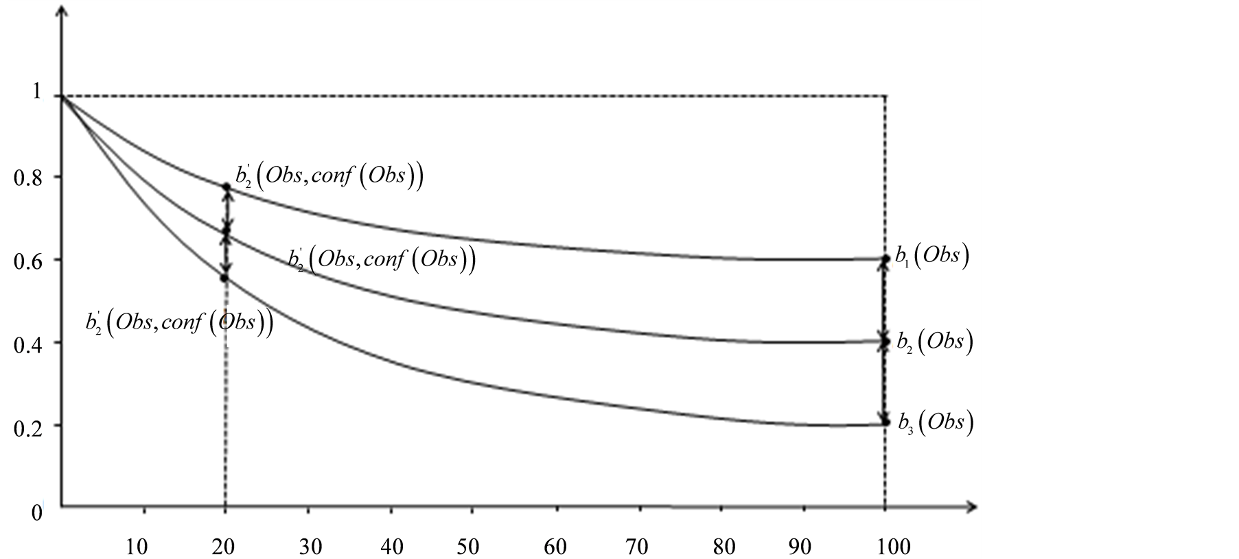
Figure 3.
 for different values of
 , with respect to
 . The x axis represents
 .
.
2.3. Use of Self Organizing Maps with Hidden Markov Models
In order to build the HMM to model such a problem, it is necessary to discretize the dynamical model outputs into a discrete set of states. This can be a complicated task. A common method which is used in cases were the dynamical model can be described with few states, is to create independent states by clustering the available data [12] . A way to cluster the data is to reduce the dimension of the problem by using a Principal Component Analysis (PCA) [13] , and then make use of Learning Vector Quantization to generate states of the HMM [14] . However reducing of the dimension of the data through a PCA, would hinder the reconstruction of highly multidimensional vectors, and would not permit a fine discretization of the data, which is important in time-series completion. In our method we use Self-Organizing Topological Maps (SOM) which are clustering methods based on neural networks [15] . They provide a discretization of a learning dataset into a reduced number of subsets, called classes, which share some common statistical characteristics. Each class corresponds to an index. For each class, the hidden data attributed to it is represented by a referent vector, which approximates the mean value of the elements belonging to it. These referent vectors are used to label any other data of the same dimension with the index of the “nearest” referent vector. The indexes represent the states of the HMM and their referent vectors are used to generate sequences of indexes of states that serve to learn the emissions and transition probabilities.
The SOM training algorithm forces a topological ordering upon the map, and therefore any neighboring classes have referent vectors that are close in the Euclidean sense in the data space. This particularity is used by PROFHMM, and by extension by PROFHMM_UNC, to improve the emissions and transitions probabilities of the HMM. It permits the inclusion of a high number of states in the HMM modeling of a phenomenon for which we have relatively few concurrent hidden and observable vectors. The process of improving these probabilities is detailed in the Appendix.
3. Application
PROFHMM_UNC can be applied to real-world data for which we have a model that is consistent with the observed quantities. However, for the scope of this article we chose to perform a twin experiment with the outputs of the NEMO-PISCES model [10] , which allow us to present the general behavior and some quantified performances of the PROFHMM_UNC. Doing so we can control the behavior of PROFHMM_UNC for different situations: low or high confidence.
3.1. The Model
NEMO-PISCES is an ocean modeling framework which is composed of “engines” nested in an “environment”. The “engines” provide numerical solutions of ocean, sea-ice, tracers and biochemistry equations and their related physics. The “environment” consists of the preand post-processing tools, the interface to the other components of the Earth System, the user interface, the computer dependent functions and the documentation of the system. We obtained the output of this model by running the ORCA2_LIM_PISCES version of NEMO, which is a coupled ocean/sea-ice configuration based on the ORCA tripolar grid at 2˚ horizontal resolution forced with climatological forcing (winds, thermodynamic forcing) in conjunction with the PISCES biogeochemichal model [10] .
We extracted the five-day averaged outputs of this model at the grid points representing the BATS station (32 N - 64 W), shown in Figure 4. This station is one of the model calibration sites due to the existence of the Bermuda Atlantic Time Series (BATS) of the JGOFS campaign [12] . From the available data, we processed the values of the Sea Surface Temperature (SST), Sea Surface Chlorophyll-A (SCHL), Wind Speed (WS), the incident Shortwave Radiation (SR) and Sea Surface Elevation (SSH), averaged every five days. These averaged time steps are denoted tNEMO. This gave us a complete data set of these five parameters for 1239 tNEMO time-steps spanning from 1992 to 2008. We then generated a matrix containing the mean value of these parameters averaged for three consecutive tNEMO time-steps. This average corresponds to the mean values of the parameters for a fifteen consecutive-days period, denoted tHMM. The data set containing the values of the five “observable” parameters at the different tHMM time-steps is noted Datahid and is a five-dimensional matrix with 413 tHMM time-steps.
In order to generate the observable situations and to simulate satellite data, we added to each geophysical parameter at the tNEMO temporal resolution, a white noise following a Gaussian N (0, 0.35 * σparam), where σparam is the standard deviation of each parameter. The data was then once more averaged every 3 consecutive tNEMO time steps, in order to reach the tHMM temporal resolution. This generated the Dataobs matrix.
3.2. Statistical Learning and Weighting Function Configuration
The SOM map (denoted sMaphid in the following) providing the hidden states of the HMM was trained with Datahid. As described in Section 2.3, by classifying the Datahid vectors, we generated a sequence of indexes, denoted SIhid. These indexes correspond to the hidden states of the model at these consecutive tHMM time-steps.
The SOM map (denoted sMapobs in the following) providing the observable states of the HMM was trained with Dataobs. Since the generation of Dataobs included the calculation of the mean value at the tNEMO temporal resolution, the white noises added to the signal is smoothed. Dataobs is a five-dimensional data set (containing SCHL, SST, SSH, WS, SR) with 413 rows. The sequence of indexes of the observable data, SIobs coincides temporally with SIhid, and was generated by classifying the Dataobs vectors.
The generation of the hidden and observable states was done by using the two SOMs. Both sMaphid and sMapobs contain 108 neurons that represent, respectively, the hidden and observable states of the HMM, distributed on an array formed of 12 by 9 lattices. They were generated using Datahid and Dataobs from 1992 to 2005, each data set corresponding to 340 tHMM time steps; the sequence of observations from the year 2006, corresponding to 24 tHMM time steps, were used as a validation set, and the years 2007 and 2008, corresponding to a sequence of 49 tHMM time steps, were used to test the performance of the method.
The size of the maps were set by iteratively increasing the number of states of each map, selecting the dimensions that had the smallest root mean square (RMS) errors between the actual data of the validation year 2006 and its reconstruction by PROFHMM.
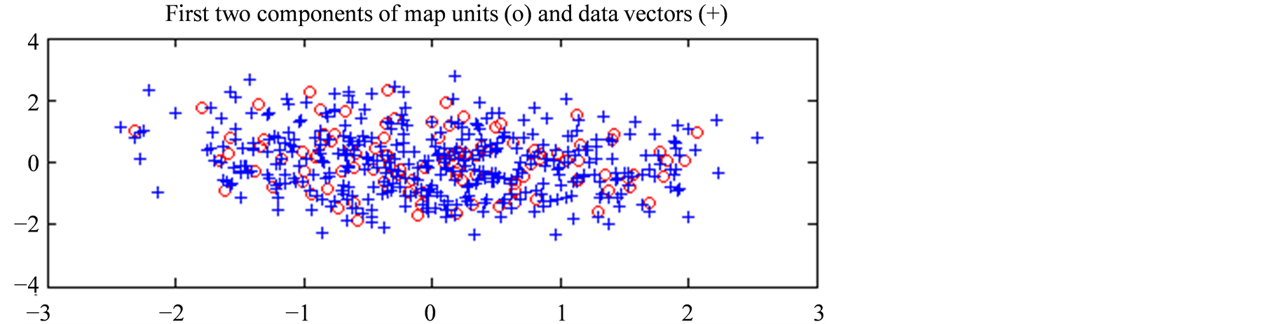
In Figure 5(a) we present, projected on the first plane given by the PCA of Datahid, the spatial distribution of the referent vectors of the hidden states as red circles, while the blue crosses correspond to the data vectors from Datahid. Similarly, in Figure 5(b) we present, projected on the first plane of the PCA of Dataobs, the spatial distribution of the referent vectors of the hidden states as red circles, while the blue crosses correspond to the data vectors from Dataobs. The first plane of the PCA of the hidden data set corresponds to 69.3% of its variance, while the first plane of the PCA of the observable data set corresponds to 68.2% of its variance. Both hidden and observable states are well distributed over their respective data set. Therefore we can make the assumption that the selected states represent accurately the variance of the observed phenomenon. It is important to note that this is just a projection of the data on the first plane and that we did not reduce the dimension of our vectors by applying this PCA.
The SOM maps were trained with the algorithms provided by the matlab som toolbox [15] , specifically the functions som_make, som_batchtrain, som_bmus in order to train our maps and classify our data.
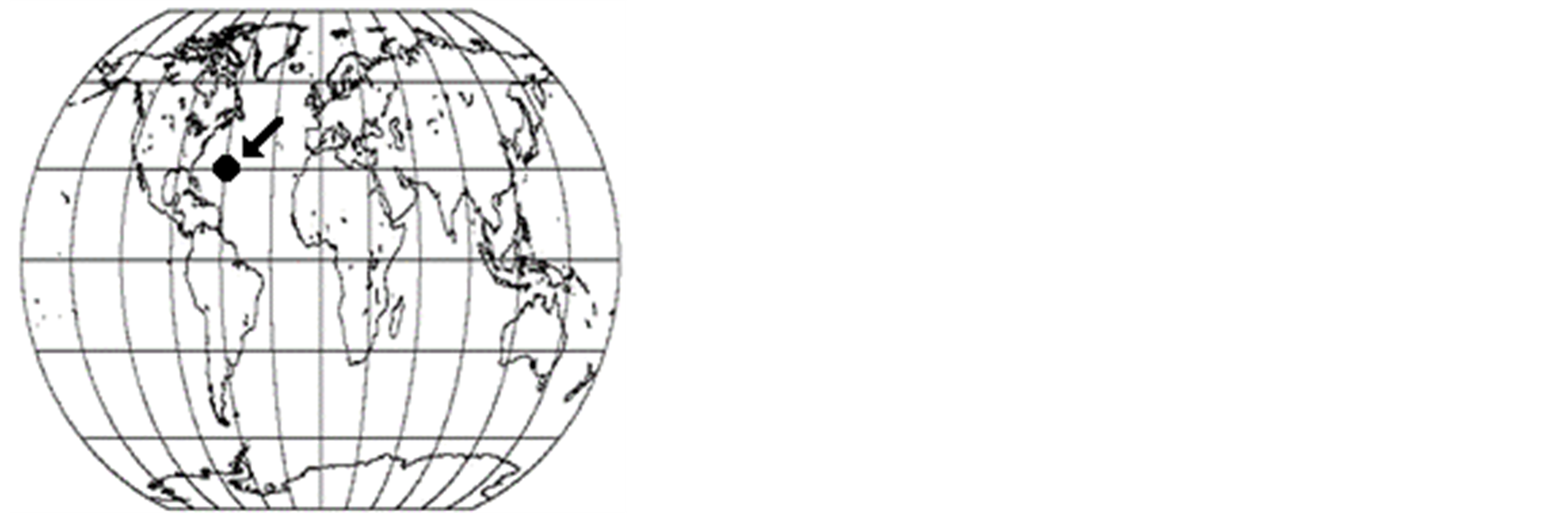
Figure 4. The location of BATS.
 (a)
(a)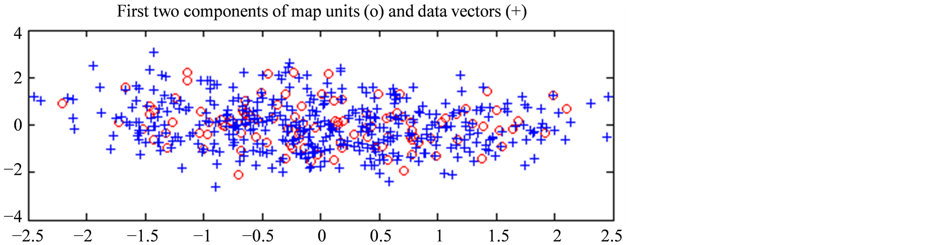 (b)
(b)
Figure 5. (a) Projection of the temperature profiles (in blue crosses) and the referent vectors of sMaphid (in red circles), onto the first plane of the PCA of Datahid; (b) Respectively, projection of the observation vectors (in blue crosses) and the referent vectors of sMapobs (in red circles), onto the plane determined by the two first eigenvectors of the PCA of Dataobs.
The SOM maps were used to classify the datasets and generate two sequences of state indexes, SIobs and SIhid. These sequences were subsequently used to train the Hidden Markov Model according to the procedure presented in Section 2, and to estimate the HMM parameters.
The weighting function was set to
 whose form can be seen in Figure 3. The determination
of the form of this function and the specific values for the exponential, was a
modeling choice made to force a slight degradation of
whose form can be seen in Figure 3. The determination
of the form of this function and the specific values for the exponential, was a
modeling choice made to force a slight degradation of
 for high
 , while greatly increasing
them for very low ones.
, while greatly increasing
them for very low ones.
We made the assumption that, due to exterior factors such as heavy cloud coverage or satellite instrument malfunction, only during some (or none) of these time-steps there were observations available. The confidence function was therefore defined as the percentage of available time-steps used to generate the observation. The flowchart of PROFHMM_UNC for the twin experiment is shown in Figure 6.
3.3. Performances
To test the performances of the model, we classified the hidden and observable data
from the years 2007 and 2008 according to their respective sMaps. However, we simulated
a perturbed sequence of data for which we introduced exterior indicators of confidence:
for twelve consecutive tHMM time steps we considered that the observable
data was not given from the mean of three consecutive tNEMO time steps,
but by the value of only one of these. Doing so we increased the noise level of
those specific data points. Therefore, an empiric way to set the confidence value
 at approximately a third of the maximum confidence,
 , since we sampled the data at the rate of one out
of the three consecutive time-steps.
, since we sampled the data at the rate of one out
of the three consecutive time-steps.
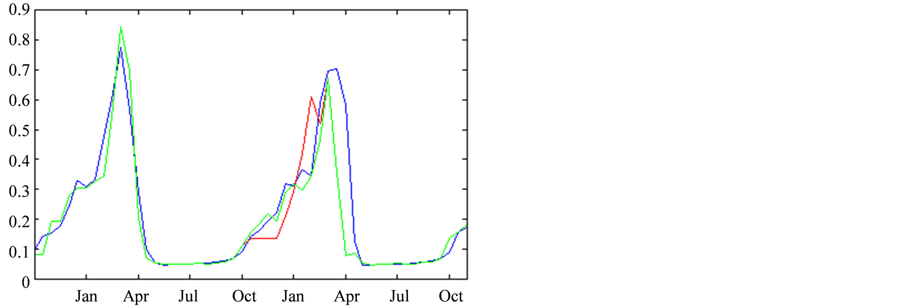
The twelve consecutive time-steps data shown in Figure
7, correspond to a period spanning from October 2007 to March 2008. We focused
on the reconstruction of the Chlorophyll-A, in Figure 7(a)
and the temperature, in Figure 7(b). The curves
in this figure correspond to the reconstructions: in red for a complete confidence
 in the observations and in green for the aforementioned
 . The real model values
are in blue. We can see that, by applying the PROFHMM_UNC, we increased our trust
in the transitions probabilities of the HMM and better fitted the curve of the real
data.
. The real model values
are in blue. We can see that, by applying the PROFHMM_UNC, we increased our trust
in the transitions probabilities of the HMM and better fitted the curve of the real
data.
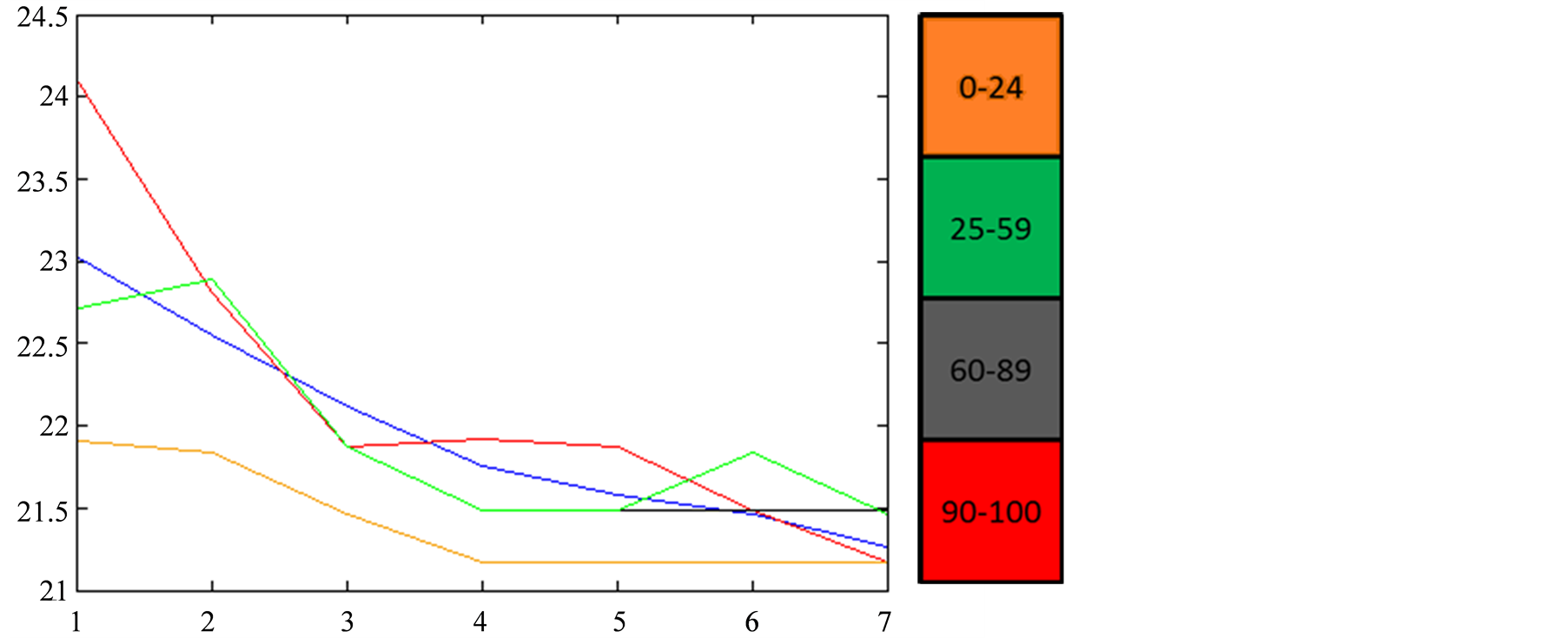
After presenting these results, we progressively varied the value of
 by increments of 5, and plotted the resulting curves of CHL and SST for the 7 tNEMO
time step period which had their sampling modified. As seen in
Figure 8, we only obtain 5 different curves when performing this experience.
In orange, we can see that if we give zero to small confidence in the data
by increments of 5, and plotted the resulting curves of CHL and SST for the 7 tNEMO
time step period which had their sampling modified. As seen in
Figure 8, we only obtain 5 different curves when performing this experience.
In orange, we can see that if we give zero to small confidence in the data , we obtain a curve that
almost does not take into account the observations and chooses the hidden states
based on transitions only. The reconstruction therefore is far away from reality.
In green we have the result obtained when we have a small, but not null confidence
in the observations
, we obtain a curve that
almost does not take into account the observations and chooses the hidden states
based on transitions only. The reconstruction therefore is far away from reality.
In green we have the result obtained when we have a small, but not null confidence
in the observations , this curve is closer
to the NEMO values. In black, we have the values obtained with a higher confidence
in the data
, this curve is closer
to the NEMO values. In black, we have the values obtained with a higher confidence
in the data . The black curve follows
the NEMO-PISCES values quite well; is hidden by the green curve up to the fifth
time step, then approximates the real data slightly better. Finally when we completely
trust the data,
. The black curve follows
the NEMO-PISCES values quite well; is hidden by the green curve up to the fifth
time step, then approximates the real data slightly better. Finally when we completely
trust the data,
 the model takes too much into account the modified
observed data, increasing therefore the error of the reconstruction.
the model takes too much into account the modified
observed data, increasing therefore the error of the reconstruction.
It is interesting to note that there are only 5 curves obtained when varying the
values of . This is due to the way
the Viterbi Algorithm functions, whose principle is to select the optimum path:
slight changes in the values of confidence will create slight modifications, which
are often not enough to overcome a threshold value needed to change the index of
the selected state, therefore generating the same path. The choice of the form of
family of functions
. This is due to the way
the Viterbi Algorithm functions, whose principle is to select the optimum path:
slight changes in the values of confidence will create slight modifications, which
are often not enough to overcome a threshold value needed to change the index of
the selected state, therefore generating the same path. The choice of the form of
family of functions
 controls the speed of the decrease of the impact of the a priori emissions probabilities
on the selection of the optimum path by the Viterbi Algorithm. This, in turn also
changes the length and placement of the intervals of
controls the speed of the decrease of the impact of the a priori emissions probabilities
on the selection of the optimum path by the Viterbi Algorithm. This, in turn also
changes the length and placement of the intervals of
 values that present the same reconstruction.
Figure 8 also raises another important point on
the determination of the
 function. In the experiment above, we initially considered an empirical value of
35, trying to approximate the fact that we only sampled the data at the rate of
one out of the 3 tNEMO time steps. This was equivalent to assuming that
they were independently selected using a simple probability distribution. However,
as seen in Figure 8, the results obtained in the
interval
function. In the experiment above, we initially considered an empirical value of
35, trying to approximate the fact that we only sampled the data at the rate of
one out of the 3 tNEMO time steps. This was equivalent to assuming that
they were independently selected using a simple probability distribution. However,
as seen in Figure 8, the results obtained in the
interval
 better fitted the data. This happens because the tNEMO time step sampling
is strongly correlated with the two ignored ones, and its associated data value
contains a significant percentage of the total information we would have obtained
by sampling all of the time steps. Therefore, it is important to perform a preliminary
study to determine the confidence function that best fits the problem. This is especially
true in the cases for which PROFHMM_UNC could be applied, since spatial and temporal
sampling at different resolutions is often encountered in different fields of study,
such as geophysical problems related to satellite information.
better fitted the data. This happens because the tNEMO time step sampling
is strongly correlated with the two ignored ones, and its associated data value
contains a significant percentage of the total information we would have obtained
by sampling all of the time steps. Therefore, it is important to perform a preliminary
study to determine the confidence function that best fits the problem. This is especially
true in the cases for which PROFHMM_UNC could be applied, since spatial and temporal
sampling at different resolutions is often encountered in different fields of study,
such as geophysical problems related to satellite information.
In order to present a quantifiable measure of the improvement obtained by applying PROFHMM_UNC, we performed a dedicated test by generating 10.000 different Dataobs. This was done while varying the placement of the consecutive 7 tHHM time steps period of low confidence throughout the 2 testing year period. The Dataobs matrices were generated by adding a, significantly stronger, white noise, that follows N (0, 1.5 * σparam) distribution, to the Datahid. We then calculated, for the years 2007-2008 the RMS errors between the reconstructed and NEMO outputs of the sea surface chlorophyll-a and sea surface temperature for each confidence interval. The results are shown in Table1
The values obtained indicate an improvement when taking into account the uncertainty
of the observations. Once more we can see that, by applying
 the results are globally improved. This
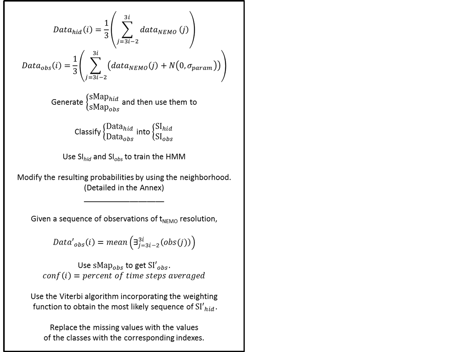
Figure 6. The flowchart
of the twin experiment. The expression
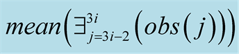 must be read as: “compute the mean for the existing values in the time sequence
from
must be read as: “compute the mean for the existing values in the time sequence
from
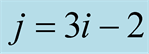 to
to .
.
 (a)
(a)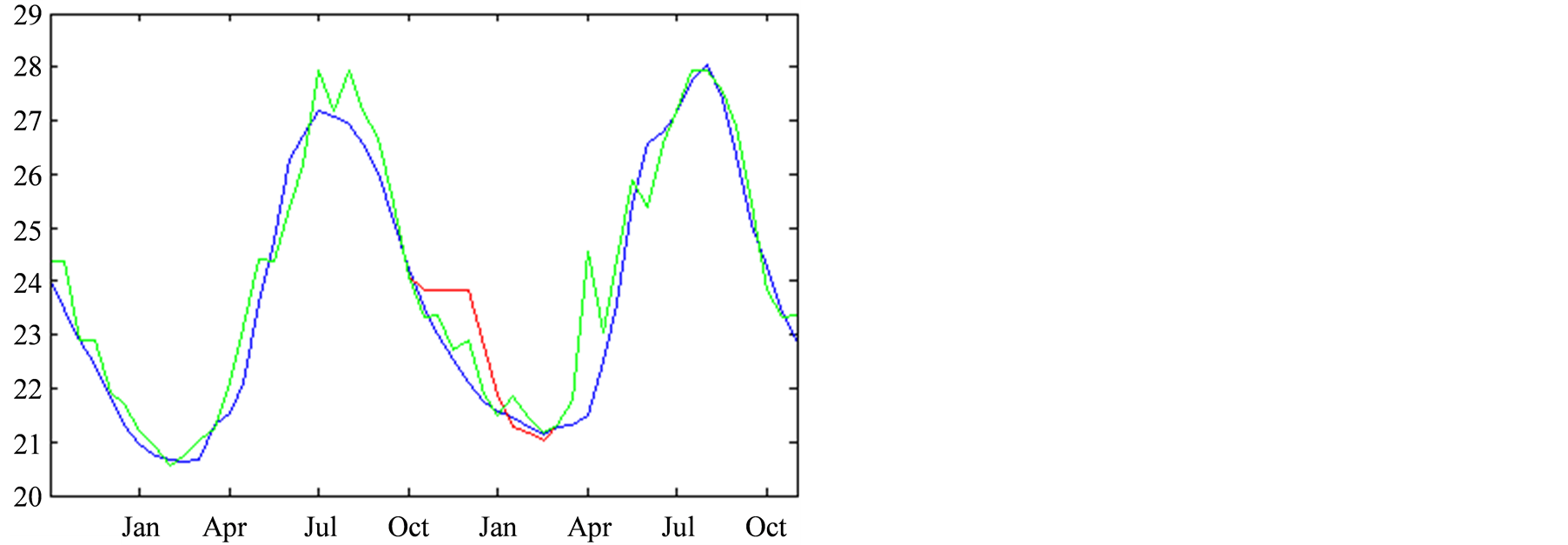 (b)
(b)
Figure 7. Reconstruction, for the years 2007 and 2008, of Sea Surface Chlorophyll-A (a), in [10−6 mg/L] and Sea Surface Temperature (b), in ˚C. The blue line corresponds to the unmodified data of Datahid. The red one corresponds to the values of the reconstruction while using the HMM without a modification of the emission probability, considering that the modified observations have a confidence of 100. The green one corresponds to the result obtained by using PROFHMM_UNC, and using a confidence of 35 for each observation between, October and March. Out of that time period, the two curves coincide and we cannot differentiate the green and red curve.
 (a)
(a)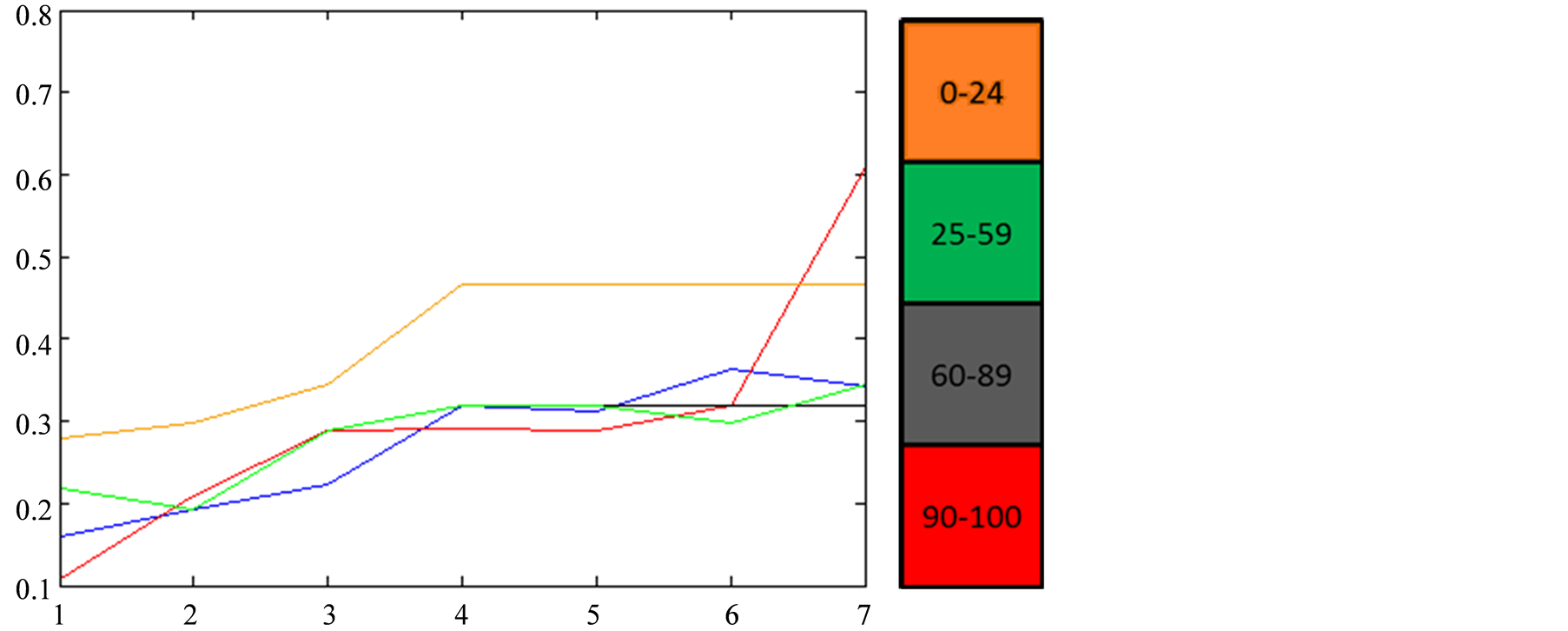 (b)
(b)
Figure 8. Variation of the reconstructed values of Sea Surface
Chlorophyll-A (a) and Sea Surface Temperature (b) with respect to the value of the
 function, for a 7 tHMM period (from October 2007 to the first half of
January 2008) assuming that each tHMM observation is computed from a
single tNEMO. In blue we have the actual values of the model. The colorbar
indicates the valued of
function, for a 7 tHMM period (from October 2007 to the first half of
January 2008) assuming that each tHMM observation is computed from a
single tNEMO. In blue we have the actual values of the model. The colorbar
indicates the valued of .
.
highlights the importance of performing a preliminary study to determine the appropriate confidence function for each phenomenon.
There exist variations of the Viterbi algorithm such as Lazy Viterbi [16] and the Soft Output Viterbi [17] [18] . We limited ourselves to the Viterbi Algorithm, yet the modification could easily be applied to those approaches.
4. Conclusions
In this paper we have presented PROFHMM_UNC, a new methodology that combines a dynamic model and observations in order to constrain the outputs of a dynamic model to better fit the observations, while respecting the dynamic processes of the model. This was used to complete time-sequences with missing data, and to correct observations for which we have an external indicator of unreliability. The improvements obtained by using the method were illustrated through a twin experiment. The results of this experiment highlight the importance of performing a preliminary study to determine a case-appropriate confidence function. PROFHMM_UNC is very general and could be applied to model a system which is not described numerically, by learning the dynamic processes using a large amount of sequences of observations.
Going forward we might intend to apply this methodology for generating realistically complete time series of states, based on real satellite observations, to further be used by PROFHMM in order to retrieve 3D fields of parameters based on discrete observations generated by PROFHMM_UNC.
Acknowledgements
The research presented in this paper was financed by Centre National de l’Etude Spatial (CNES, French national center of spatial studies), and the Delegation Gouvernemantale pour l’Armement (DGA, French Military Research Delegation), which we wish to thank for their support. We wish to also thank Cyril Moulin and Laurent Bopp from LSCE for their help with NEMO-PISCES and Michel Crepon for his input on the method.
References
- Dempster, A.P., Laird, N.M. and Rubin, D.B. (1977) Maximum Likelihood from Incomplete Data via the EM Algorithm. Journal of the Royal Statistical Society. Series B, 39, 1-38.
- Ghahramani, Z. and Jordan, M.I. (1994) Supervised Learning from Incomplete Data via an EM Approach. Advances in Neural Information Processing Systems (NIPS 6), Morgan Kauffman, San Fransisco, 120-127.
- Wasito, I. and Mirkin, B. (2005) Nearest Neighbour Approach in the Least-Squares Data Imputation Algorithms. Information Sciences, 169, 1-25.
- Chiewchanwattana, S., Lursinsap, C. and Chu, C.-H.H. (2007) Imputing Incomplete Time-Series Data Based on Varied-Window Similarity Measure of Data Sequences. Pattern Recognition Letters, 28, 1091-1103. http://dx.doi.org/10.1016/j.patrec.2007.01.008
- Prasomphan, S., Lursinsap, C. and Chiewchanwattana, S. (2009) Imputing Time Series Data by Regional-Gradient-Guided Bootstrapping Algorithm. Proceedings of the 9th International Symposium on Communications and Information Technology, Incheon, 163-168.
- Grayzeck, E. (2011) National Space Science Data Center, Archive Plan for 2010-2013. NSSDC Archive Plan 10-13.
- Robinson, A.R. and Lermusiaux, P.F.J. (2000) Overview of Data Assimilation. Harvard Reports in Physical/Interdisciplinary, Ocean Science, No. 62.
- Viterbi, A.J. (1967) Error
Bounds for Convolutional Codes and an Asymptotically Optimum Decoding
Algorithm. IEEE Transactions on Information Theory, 13, 260-269. http://dx.doi.org/10.1109/TIT.196
7.1054010 - Charantonis, A.A., Brajard, J., Moulin, C., Bardan, F. and Thiria, S. (2011) Inverse Method for the Retrieval of Ocean Vertical Profiles Using Self Organizing Maps and Hidden Markov Models—Application on Ocean Colour Satellite Image Inversion. IJCCI (NCTA), 316-321.
- Jaziri, R., Lebbah, M., Bennani, Y. and Chenot, J-H. (2011) SOS-HMM: Self-Organizing Structure of Hidden Markov Model, Artificial Neural Networks and Machine Learning—ICANN 2011. Lecture Notes in Computer Science, 6792, 87-94. http://dx.doi.org/10.1007/978-3-642-21738-8_12
- Madec, G. (2008) NEMO Ocean Engine. Note du Pole de modélisation, Institut Pierre-Simon Laplace (IPSL), France.
- Willsky, A.S. (2002) Multiresolution Markov Models for Signal and Image Processing. Proceedings of the IEEE, 90, 1396-1458. http://dx.doi.org/10.1109/JPROC.2002.800717
- Jolliffe, I.T. (2002) Principal Component Analysis. 2nd Edition, Springer, Berlin.
- Kwan, C., Zhang, X., Xu, R. and Haynes, L. (2003) A Novel Approach to Fault Diagnostics and Prognostics. Proceedings of the 2003 IEEE International Conference Robotics & Automation, Taipei.
-
Kohonen, T. (1990) The Self-Organizing Map. Proceedings of the IEEE, 78.
http://www.cis.hut.fi/projects/somtoolbox/package/docs2/somtoolbox.html -
Doneya, S.C., Kleypasa, J.A., Sarmientob, J.L. and Falkowski, P.G. (2002) The US
JGOFS Synthesis and Modeling Project—An Introduction. Deep-Sea Research II, 49,
1-20.
http://dx.doi.org/10.1016/S0967-0645(01)00092-3 -
Viterbi, A.J. (1998) An Intuitive Justification and a Simplified Implementation
of a MAP Decoder for Convolutional Codes. IEEE Journal on Selected Areas in Communications,
16, 260-264.
http://dx.doi.org/10.1109/49.661114 - Hagenauer, J. and Hoeher, P. (1989) A Viterbi Algorithm with Soft-Decision Outputs and Its Applications. IEEE Global Telecommunications Conference and Exhibition “Communications Technology for the 1990s and Beyond” (GLOBECOM), 1680-1686.
Appendix
Advantages of Using Self-Organizing Maps for the Determination of HMM States
Self-Organizing Topological Maps (SOM) which are clustering methods based on neural networks. They provide a discretization of a learning dataset into a reduced number of subsets, called classes, which share some common statistical characteristics. Each class is represented by a referent vector, which approaches the mean value of the elements belonging to it, since the training algorithm can be forced to perform like the K-means algorithm at the final stages of its training.
The topological aspect of the maps can be justified by considering the Map as an undirected graph on a twodimensional lattice whose vertices are the classes. This graph structure permits the definition of a discrete distance, noted d, between two classes, defined as the length of the shortest path between them on the map.
Any vector that is of the same dimensions and nature as the data used to generate the topological map, can be classified by assigning it to the class whose referent it resembles most. Therefore a sequence of data vectors can be classified in order to generate a sequence of indexes that correspond to the indexes of the classes to which they were assigned.
In our method, we trained two SOMs, the first containing the observations, called sMapobs and the second containing the hidden states, called sMaphid. The hidden states correspond to the discretization of the numerical dynamic model.
The classes of sMapobs and sMaphid correspond respectively
to the discretization of the observation vectors into a set amount of observable
states,
 , and to the hidden states of the HMM,
 .
.
The topological aspect of the SOMs is useful in overcoming the usual lack of sufficient data in estimating the transition and emission probabilities of the HMM. After an initial estimation of the probabilities over each available training sequence, noted seq, these transitions, Trseq, and emissions Emseq, can be combined and adjusted by taking into account the neighboring properties of the topological maps.
This is done by considering the neighborhood matrices NMobs and NMhid,
of dimensions
 and
and
 respectively, where
 , (1)
, (1)
with
 being the discrete distance on the respective maps.
The final Em and Tr matrices we used, noted Emfinal and Trfinal,
were computed by applying for
 and for
 :
:
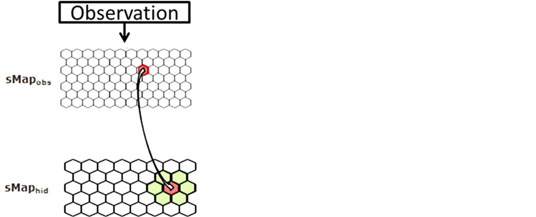
Figure A1. The emission probability of each class Yk of the sMapobs is emitted from a class Xi of sMaphid that takes into account the probability of being emitted by a class Xj neighboring Xi.
 , (2)
, (2)
Which was normalized to become
 where
where for
for

 , (3)
, (3)
which is normalized to become
 where
where .
.
The term
 corresponds to a weighting constant that prevents the actual measured probabilities
from being overshadowed by their neighborhood values. Its value is determined by
an iterative optimization process on an independent test data set. In the case of
the application (Section 3.2) its value is taken to be equal to 9. The impact of
neighboring states on the probabilities has been schematized in
Figure A1.
corresponds to a weighting constant that prevents the actual measured probabilities
from being overshadowed by their neighborhood values. Its value is determined by
an iterative optimization process on an independent test data set. In the case of
the application (Section 3.2) its value is taken to be equal to 9. The impact of
neighboring states on the probabilities has been schematized in
Figure A1.
It is important to retain that in order to apply PROFHMM_UNC, we require a training data set of concurrent hidden and observable states sequences. This, unlike more complicated cases of HMMs (such as voice recognition software), permits for an estimation of the initial emissions and transition probabilities through the use of a counting algorithm such as hmmestimate of the matlabstat_toolbox.