Journal of Water Resource and Protection
Vol.5 No.8(2013), Article ID:35842,12 pages DOI:10.4236/jwarp.2013.58083
Regional Mapping of Vertical Hydraulic Gradient Using Uncertain Well Data: A Case Study of the Toyohira River Alluvial Fan, Japan
1Division of Earth and Planetary Dynamics, Faculty of Science, Hokkaido University, Sapporo, Japan
2Geotechnical Department, Division of Environmental Engineering, Docon, Sapporo, Japan
Email: *yoshitaka_sakata@mail.sci.hokudai.ac.jp
Copyright © 2013 Yoshitaka Sakata, Ryuji Ikeda. This is an open access article distributed under the Creative Commons Attribution License, which permits unrestricted use, distribution, and reproduction in any medium, provided the original work is properly cited.
Received May 24, 2013; revised June 27, 2013; accepted August 1, 2013
Keywords: Vertical hydraulic gradient; Groundwater flow system; Alluvial fan; Kriging; Recharge; River leakage; Urbanization
ABSTRACT
Vertical hydraulic gradient (VHG) provides detailed information on 3D groundwater flows in alluvial fans, but its regional mapping is complicated by a lack of piezometer nests and uncertainty in conventional well data. Especially, determining representative depth of well screen in each well is problematic. Here, a VHG map of the Toyohira River alluvial fan, Sapporo, Japan, is constructed based on groundwater table elevation (GTE), using available well-data of various screen lengths and depths. The water-level data after 1988, when subway constructions are mostly completed in the city, are divided into those of shallow wells (≤20 m deep), and those of deep wells (>20 m deep). First, the GTE map is generated by kriging interpolation of shallow well data with topographic drift. Next, the individual VHG value of each deep well is calculated using its top, middle, and bottom elevations of the screen depths, respectively. The VHG maps of three cases are then obtained using neighborhood kriging. The VHG map of the bottom screen depths has proven most valid by cross-validation. The VHG map better visualizes that downward flows of groundwater are predominant over the fan. Positive area of VHG is mostly vanished around the fan-toe, indicating urbanization effect such as artificial withdrawals. A negative peak of VHG corresponds to recharge area, and is seen along the distinct losing section in the river. The negative peak also expands upstream to the fan-apex where a basement is suddenly depressed.
1. Introduction
Alluvial fans are typically important as groundwater reservoirs owing to high-permeability of gravel deposits [1]. Alluvial fans are found at the foot of a range of hills or mountains over the world, especially in aridand semiarid regions where sparse vegetation and occasional intense rainfall promote aggradation of coarse deposits [2, 3]. In such areas of high evaporation, alluvial fans provide groundwater storages that can be managed to increase the useful water resource. However, the extent of deposits is usually limited in area, and so the groundwater capacity is not inexhaustible. In addition, the gravel deposits are susceptible to excessive withdrawals by pumping wells or underground constructions. It might follow that ground-subsidence or water-pollution increasingly occurs. Also in grown-up fans, a rapid recovery of groundwater-table might do damages to the underground infrastructures, which was constructed during the drawdown period of the groundwater potential [4]. Recent study in Japan suggests that future climate change might significantly influence on groundwater vulnerability in alluvial fans [5].
Alluvial fans usually show moderate extent of land, e.g., several to tens square kilometers, but hydraulic head in the fan is spatially variable no less than in more wider regional sites, due to topographic, geologic and hydrologic features [1]. Surface water usually infiltrates into the ground at the fan-apex to the mid-fan, resulting in downward flow of groundwater into the deeper zone. The constituent materials gradually increase in fineness, and interbedded fine layers may divide the aquifer into unconfined and several confined layers. The confined water moves down, and is discharged when the pressure surface is higher than the ground surface. Unconfined water also emerges to the point where the water table intersects the surface. The combined discharge usually makes springs and swamps around the fan-toe. Thus, groundwater flow system in an alluvial fan is characterized by upward and downward flows of groundwater, and so understanding of the complex system requires regional information on vertical flows over the fan.
Vertical hydraulic gradient (VHG) is generally used for delineating the direction and magnitude of vertical groundwater flows [6]. Theoretically, hydraulic gradient can be calculated by derivation of hydraulic head. In-situ measurement of VHG is performed using piezometer nests, which contain multiple piezometers in close proximity at different depths. However, installing piezometers is expensive and time-consuming. Thus, the number of piezometers at a particular site is usually limited, and piezometer nests are even less frequently made. For these reasons, VHG maps are often produced, but are typically limited to a relatively local area, such as fluvial channels (for quantifying surface/groundwater interaction) and polluted sites (for monitoring contaminant plume). On a wider regional scale, VHG mapping is rarely performed, and delineation of regional groundwater flow systems is often just a 2D horizontal map with schematic vertical cross sections.
Comparable information can often be collected from the available water level data in individual water wells and boreholes. In many urbanized and developing regions, numerous records of wells and boreholes are maintained. However, such available data have been rarely used for scientific researches due to uncertainty different among individual wells. For example, uncertainty arises from differing measurement times, even in the same well, as a result of precipitation, artificial intake, climate change, and other events. Such uncertainty in each well is often calibrated based on other water variations at neighboring location and depth [7]. However, it is difficult to classify and quantify uncertainty in all of the available data. Representative depth of well screen for each water-level is probably most problematic. Water wells do not have a short single screen, but rather multiple long screens installed for water intake. The water level actually does not integrate the heads on a vertical section, depending on heterogeneity around the well [8, 9].
One traditional approach is to plot well depth versus depth to static water level from the groundwater table [6]. Under the assumption of a single topographic region, the plot determines whether the region is a recharge (downward flow) or discharge (upward flow) area. The object of this study is to expand the concept of the plot method to be more generalized on a regional scale. This study proposes regional mapping of VHG using kriging interpolation of available well data of various screen lengths and depths. The datum surface of VHG is, as in the plot method, the groundwater table (here, groundwater table elevation (GTE) in particular). Kriging is an effective interpolation tool not only for hydraulic head but also for hydraulic gradient [10]. Here, the Toyohira River alluvial fan, Sapporo, Japan, is used as a case study on VHG mapping. Available water-level data after 1988, when the subway constructions in the city are mostly completed, are grouped by well depth into those of shallow wells and of deep wells. A GTE map is first produced using the shallow well data. Individual VHG values in the deep wells are calculated from their water levels, prior estimated GTE, and representative values of screen depth elevation. Three cases, namely, the top, middle, and bottom elevations of screen, are used for addressing its uncertainty, and the VHG maps are assessed by crossvalidation. The actual groundwater flow system in the fan is examined from the resulting GTE and VHG maps.
2. Study Area: Geographic and Hydrogeological Overview
The study site is the Toyohira River alluvial fan in Sapporo, Japan (Figure 1). The Toyohira River alluvial fan is located at latitude 43˚N and longitude 141˚E, and has a radius of about 7 km and an area of about 31 km2. The fan is situated where the Toyohira River flows northward out of Tertiary mountains and debouches on a plain. The Toyohira River is about 72.5 km long and has a watershed area of about 900 km2. In this area, the annual mean precipitation between 1981 and 2010 is 1107 mm. The median value of daily mean river flows through the fan are 12.6 m3/s for the period of record 1975 - 2010; maximum instantaneous peak discharge reached 700 m3/s in August 1981. The fan is surrounded by Tertiary volcanic mountains to the west, hilly lands covered with Pleistocene volcanic deposits to the east, and lowland to the north. On the lowland, the Toyohira River confluences with the Ishikari River, one of the main rivers of Japan, and flows into the sea. The fan is a compound fan comprising a western Holocene fan at 70 - 10 m asl (above mean sea level) and an eastern Pleistocene fan at 90 - 20 m asl. The mean inclinations of both fan surfaces are also different: 9/1000 in the Pleistocene fan, 7.5/1000 in the Holocene fan. The topographic boundary between the surfaces forms as an abrupt cliff of several meters in height along the river upstream from KP 15, where KP denotes the distance in kilometers from the confluence with the Ishikari River. The Toyohira River alluvial fan developed as follows: 1) the Pleistocene fan was formed when the sea level was lower in the last glacial period; 2) as the sea level rose in the early Holocene, the Toyohira River shifted toward the west, crossing through the Pleistocene fan, and gradually formed the Holocene fan; 3) in the late Holocene, the river shifted its channel eastward as sediments were deposited, resulting in the present course of the river [11].
Figure 1 also shows over 1000 water-wells and boreholes in the city, most of which are publicly available, and a part of which are obtained from private or unpublished reports. Since the 1970s, groundwater level and quality in the fan have been monitored by the Hokkaido Regional Development Bureau and the Geological Survey of Hokkaido. The observation wells are shown as solid squares in Figure 1, and details about the wells are listed in Table 1. Furthermore, in 2010 the authors observed water levels at some of the individual wells and in a longitudinal distribution of river stages to obtain more valid data. The annual mean water variations at the observation wells are shown in Figure 2. Significant drops in water level are seen in most observation wells during 1985-1987, which are years when subway constructions occurred. Previous study performed statistical analyses for the long-term water-level variations, indicating that both daily fluctuations and annual variations after 1988 ranged within a few meters [12].
A longitudinal geologic cross section in the fan is shown in Figure 3. Tertiary volcanic formations appear beneath the riverbed at the fan head, but the fan basement suddenly inclines northward to a depth of several hundreds of meters. As a result of this depression, various Quaternary sediments-such as gravels, sand, silts, clays and humus-hundreds of meters thick underlie the mid to distal parts of the fan. Instead of base rock, Pleistocene marine sediments at –50 to –30 m asl serve as a hydrogeologic basement for the subsurface.
The upper formations are divided into four aquifers: Pleistocene nos. IV and III, and Holocene nos. II and I [13]. Consisting of alternating gravel, sand, and silt lay ers tens of meters thick, the Pleistocene no. IV aquifer formed before the development of the alluvial fan. Both
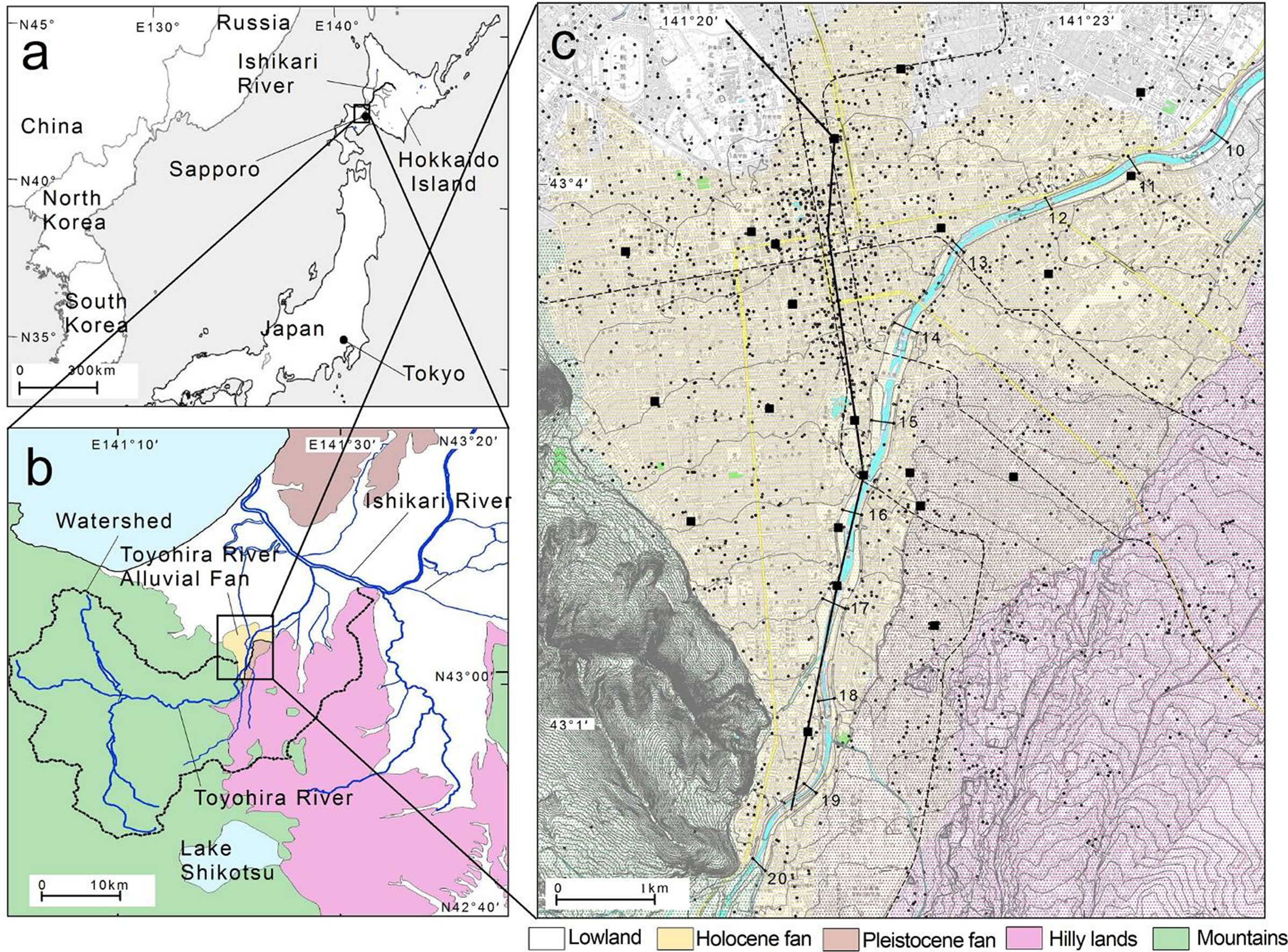
Figure 1. Location maps and topographic features of the study area: the Toyohira River alluvial fan. Small points in Figure 1c are the wells and boreholes that provided water level data before filtering (n = 1392). Solid squares are long-term observation wells, details of which are listed in Table 1. Bold black line shows the position of the cross section in Figure 3. Gray dashed lines are subway lines constructed in the city. Figure 1c also shows ground surface contours with 1 m interval from 5 to 80 m asl, and short lines along the river indicate KP which denote the distance (in kilometers) along the river channel upstream from the confluence with the Ishikari River.

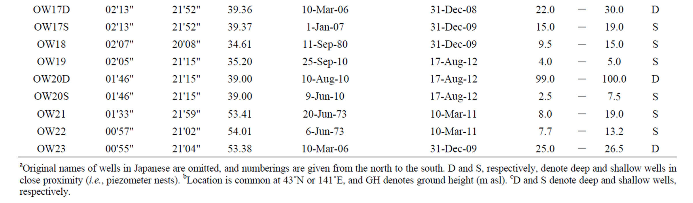
Table 1. Long term observation wells in the toyohira river alluvial fan.
the Pleistocene no. III and Holocene no. II aquifers consist mainly of alluvial fan deposits, that is, poorly sorted sandy gravel with andesitic cobbles. The total thickness of gravel aquifers is over 100 m at the upper middle of Holocene fan, and less than 50 m at the distal part. The Holocene no. I aquifer is distributed in only the northern part of the fan, and is continuous in the lowland. This aquifer consists of sandy beds, clayey beds, and peaty beds, which were transported in the late Holocene. Figure 3 also indicates potentiometric contours of groundwater head manually plotted using data from several piezometric nests. The contours show a 3D groundwater flow system in the fan; horizontally from the apex to the distal part and vertically from the ground surface to the deeper aquifer. This regional flow of groundwater in the fan is due to not only the steep fan surface, but also high rate of infiltration from the river. The estimated rate of leakage through the riverbed is approximately 1 m3/s due to a distinct losing section at KP 15.5 - 17 [14]. The infiltration also results in characteristic profiles of groundwater temperature in the wells near the river channel, with seasonal fluctuation (envelope) and deepening of isothermal layer [15].
The Toyohira River alluvial fan has characteristics of an urbanized fan. The population of Sapporo City exceeds 1.9 million, and continues to increase. Annual reports give total water well pumping rates of over 100,000 m3/day. Figure 4 shows that well depths and screen
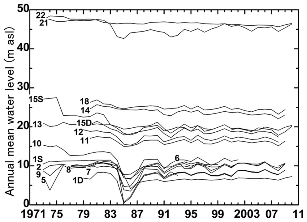
Figure 2. Long-term variations in annual mean water levels in the observation wells. Variations are produced in the observation wells from hourly data covering at least 3 years. The numbering of the observation wells is shown in Table 1.
lengths are variously distributed: most well depths range from 30 to 50 m, and the screen lengths are almost evenly distributed until 50 m. Also, underground structures such as three subway lines drain groundwater, and thus neighboring aquifers. The vulnerability of groundwater in the fan has been discussed for several decades. Furthermore, both seepage loss and water intake are believed to lower the minimum discharge necessary for sustaining life in the river, including endangered salmon. Understanding of the groundwater flow system in the fan is required for conservation and sustainable use of both surface water and groundwater.
3. Methods
3.1. Data Preparation
In this study, only post-1988 water-level data in the city are used for our analysis. The daily and annual variations of water-level are within few meters as described above, and this study determines that this range is not enough small but acceptable for this regional mapping. If multiple measurements are available at the same well, the data with the latest date are used. Automatic records, often updated hourly, are averaged over the full post-1988 measurement period.
The extracted water levels are divided into two categories: shallow wells for GTD mapping, and deep wells for VHG mapping. Groundwater levels in the shallow wells are considered to be nearly equal to the groundwater table at the time and location, because the water tables are observed initially at ≤20 m depth during the drilling of wells and boreholes in the fan. On the other hand, groundwater levels in the deep wells might be affected by VHG at the location. Consequently, the extracted water levels obtained since 1988 are divided into two categories: shallow wells of up to 20 m deep (n = 216), and deep wells of greater than 20 m deep (n = 203).
The data set is input into a geographical information system (GIS). GIS makes it feasible to interpolate environmental variables through built-in applications based on deterministic or geostatistical techniques. In this study, ArcGIS v.10 and spatial analyst tool (ESRI) are used for analysis and mapping. The target region in this study is defined in the range of the X coordinate (north-south) as −101,000 to −111,000 m and the Y coordinate (east-west) as −77,000 to −68,000 m on the Japanese Geodetic Datum 2000 (JGD2000). The extent loosely corresponded to latitude from 43˚05'13''N to 42˚59'52''N and longitude from 141˚18'15''E to 141˚24'58''E.
3.2. Kriging Interpolation
Kriging gives best linear unbiased estimator (BLUE) and its variance at any given point by using neighbor measurements and a variogram model. Maps of target variables, GTE and VHG in this study, are generated by kriging interpolation on a regular grid cell, 100 m by 100 m. The size is set based on the accuracy of well location data. The experimental variogram, which characterizes the spatial variability of the data, is defined as half the average squared difference between two attributed values. In this study, variogram modeling (i.e., production of the experimental variogram and parameterization of the theoretical variogram) is performed by using the software Surfer 10 (Golden Software).
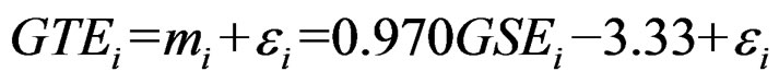
The GTE mapping is performed using regression kriging with the shallow well data, because groundwater table often relates to the ground surface linearly. In regression kriging [16], the drift and residuals are fitted separately and then summed. The formulas and parameters of drift are firstly determined by ordinary least squares (OLS). Statistically, unbiased parameters of drift are also determined by the iterative process of generalized least squares (GLS) [17,18]. GLS is a sophisticated but laborious process. The first OLS drift should be satisfactory but slightly inferior [19,20]. In this study, a simple linear relation is established between the GTE at each shallow well and its ground surface with the correlation coefficient R2 of 0.96. The GTE value is thus represented as
 , (1)
, (1)
where GTEi is the groundwater table elevation estimated at a shallow well, i is the index of the shallow well, mi is the deterministic drift derived from the topography, εi is random spatially correlated residual, and GSEi is the ground surface elevation at the shallow well. Elevation in this paper is given in meters above mean sea level.
The spatial variability of residuals, εi is estimated as a variogram model. Figure 5 shows the experimental variogram of the residuals, εi. A spherical model is used as the theoretical variogram model after a comparison
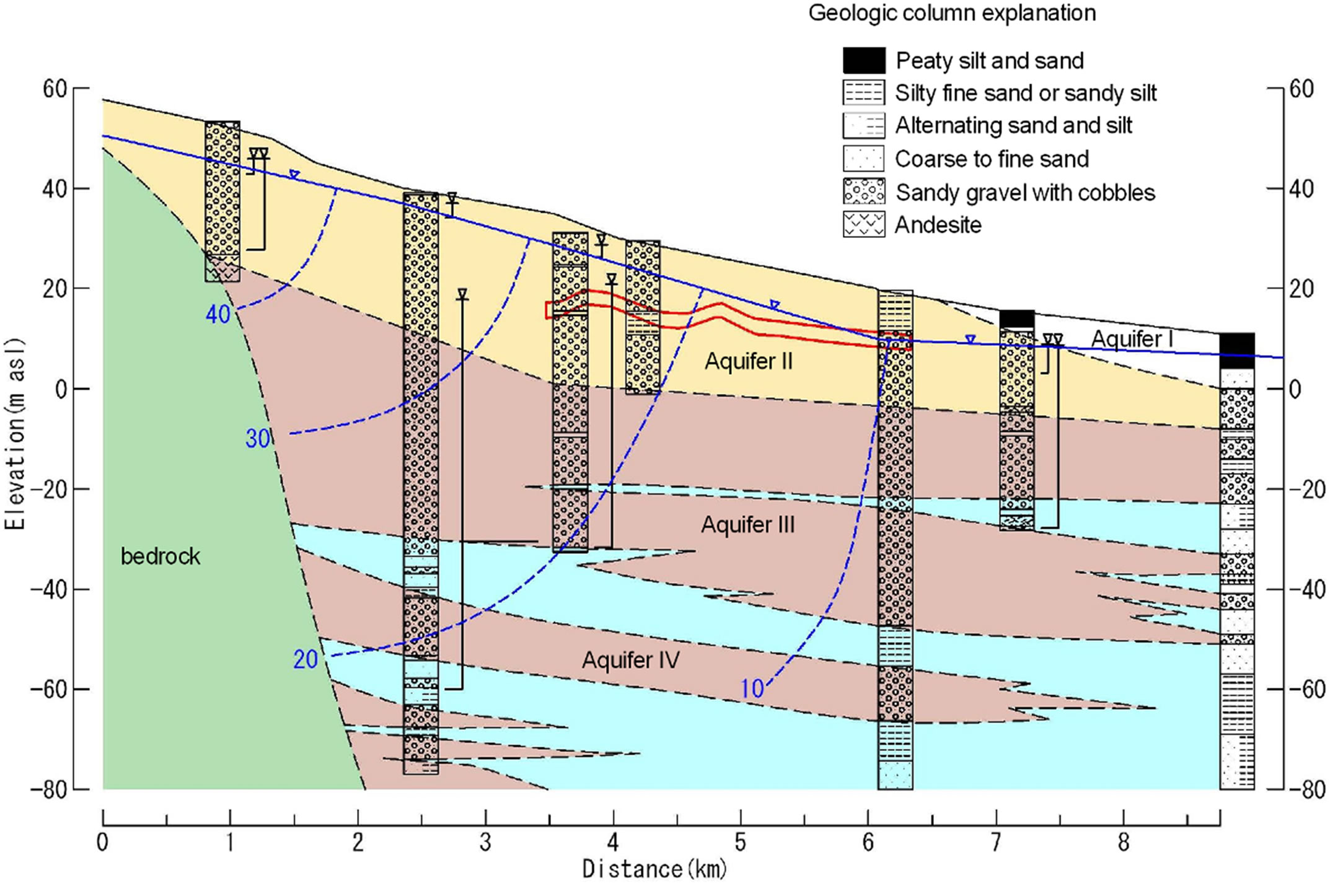
Figure 3. Geologic cross section, the Toyohira River alluvial fan. Inverted open triangles denote piezometric heads averaged during observation periods at piezometer nests. Classifications of aquifers nos. I, II, III, and IV are described in the texture. Blue solid and broken lines are, respectively, groundwater table and potentiometric contours with head elevation values (m asl). The area enclosed in red indicates the location of subway lines crossing near the section.
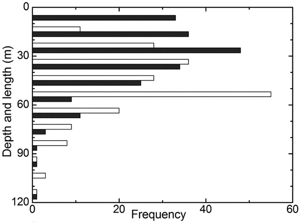
Figure 4. Histograms of well depths (open bars) and screen lengths (solid bars). Screen length is the distance from the top to bottom of screens. The wells (n = 203) are measured since 1988.
among authorized models:
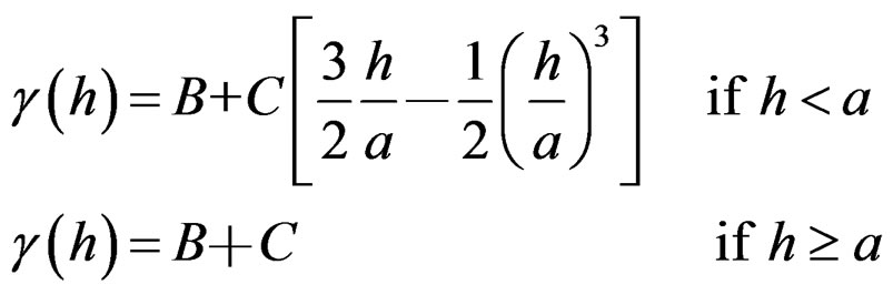 . (2)
. (2)
here, B is the nugget effect, C is the partial sill, a is the range, and h is the separation distance. Anisotropy of the spatial variability is a main consideration in hydraulic head mapping [19]. In this study, isotropy in residuals is assumed because the topographic drift extracts anisotropy, and cross-validation indicates satisfactory results as shown later. The GTE map is finally obtained by adding the residual map to the drift map. The residual map is produced by ordinary kriging assuming a stationary condition. The drift map is prepared by combining an available digital elevation map (DEM) and Equation (1). The raster calculation in GIS is used for this process. The groundwater table depth (GTD) is also mapped by subtracting the GTE map from the DEM.
Following GTE mapping, the VHG value at each deep well is calculated as
 , (3)
, (3)
where VHGj is the individual VHG value in a deep well and j is the index of the deep well. A positive (negative) value indicates upward (downward) groundwater flow. WLEj is the water level elevation, GTEj is the GTE value extracted from the prior map through the GIS application. SDEj is the representative value of screen depth elevation between the top and bottom screen depths. SDEj is considered to differ among the deep wells, and its determination is problematic. In this study, three cases, namely,
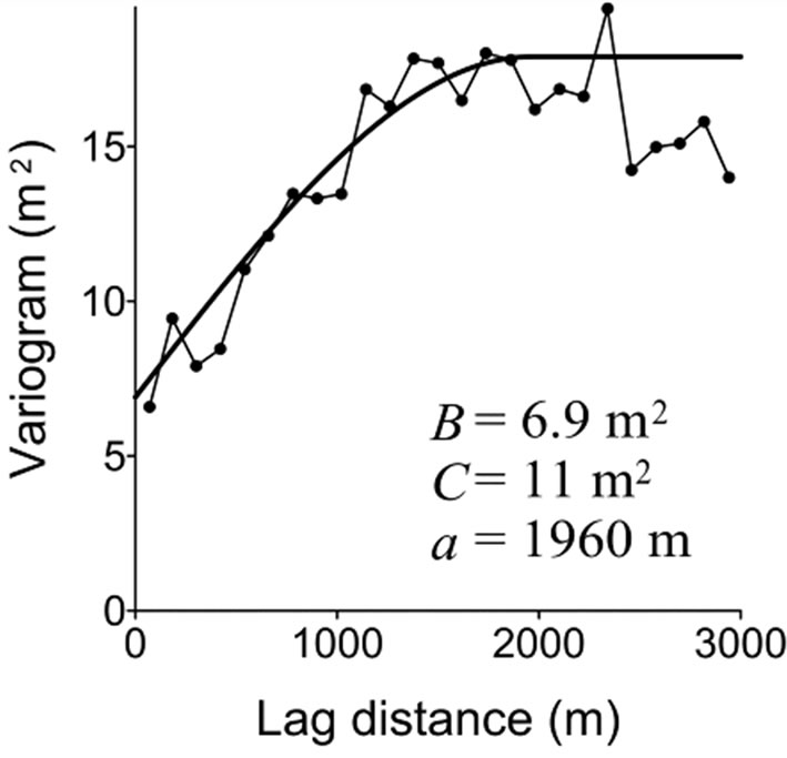
Figure 5. Omnidirectional variogram and fitted spherical model for residuals of GTEi, Optimized values of nugget B, partial sill C, and range a are indicated.
the top, middle, and bottom elevations of screens, are used for individual VHG calculation. The VHG values in the different cases are respectively mapped by ordinary kriging interpolation.
Figure 6 shows variograms of individual VHG values for three cases: the top, middle, and bottom screen depth elevations. The spherical models are used for fitting as GTE. The nugget and partial sill values are largest in the case of the top elevations, and smallest in the case of the bottom elevations. The variogram models in these cases do not converge over a distance of 2000 m, indicating the possibility of a spatial trend in VHG. Regrettably in this study, the appropriate drift of VHG is not determined although various factors such as topography, coordinates, geology are examined. Therefore, this study applies moving neighborhood kriging [21-23] in the assumption that VHG is locally stationary with a search radius of 1000 m.
3.3. Cross-Validation
Cross-validation is used to verify the resulting GTE and VHG maps. For the GTE map, cross-validation is performed for residuals at all of the shallow wells, and then the residuals are translated to GTE estimates by summing the topographic drift. The resulting GTE estimates are compared with the measurements, GTEi. For the VHG maps, cross-validation is conducted at all of the deep wells in each case of different SDEj values. The mean error (ME), root mean square error (RMSE), and mean square standard error (MSSE) are used for error estimation:
 , (4)
, (4)
 , (5)
, (5)
 , (6)
, (6)
where n is the number of wells (shallow wells for GTE mapping, or deep wells for VHG mapping), z(xi) is the measured GTE or VHG value at location xi,  is the estimated GTE or VHG using the n – 1 other data, and σi2 is the kriging standard deviation, which is the prediction error at location xi. The selected variogram model and its optimized parameters are adequate when the ME and RMSE values are close to zero, and the MSSE value is close to one with a tolerance range [
 ] [24].
4. Results and Discussion
4.1. GTE and GTD Maps
Figure 7 shows the cross-validation results of GTE mapping. The ME and MSSE values are, in large part, close to zero and one, respectively, indicating the suitability of the mapping. The RMSE value means that the prediction errors are within several meters. Such estimation errors of this level are regrettably inevitable under the uncertainty of conventional well data, owing to daily fluctuation and long-term trends. However, the errors are insignificant for discussing the GTE map on a 101 m order scale.
Figure 8 shows the estimated maps of GTE and GTD. Variance maps are omitted here, but the above cross-validation shows that the uncertainty is within acceptable limits for discussing the maps on 10 m contour scale. The steep land-surface slope of the fan contributes to the substantial driving force from the apex to the distal part. The GTE inclines northward between about 5 - 60 m asl within a distance of only about 5 km. A GTE mound and shallow GTD zone also appear along the river at KP 14 - 19, indicating the interaction between surface water and groundwater through the riverbed. The radius of the GTE mound and shallow GTD zone is no more than 1 km from the river channel. The groundwater table is deep (GTD ≥ 6 m) except around the river. In contrast to previously published water table contours before subway construction [25], the dewatering of the fan exceeds 5 m from the middle to distal parts. In the southeast part of the Pleistocene fan, the groundwater table is especially deep (GTD > 10 m), indicating an incorporation of groundwater recharge by highland and dewatering by subway lines, as also indicated in the VHG map discussed below.
4.2. VHG Map
4.2.1. Comparison among Results of Three Cases
Figures 9-11 show the obtained VHG and its variance maps in the case of the top, middle, and bottom screen depths, respectively. The spatial trend of VHG in the fan, for example negative or positive, almost corresponds among the three cases. However, the contrast of

Figure 6. Omnidirectional variogram and fitted spherical model for VHGj in three cases: (a) top, (b) middle, and (c) bottom screen depth elevations used for VHG calculation.

Figure 7. Cross-validation results of GTE above sea level.
VHG is large in the VHG map of top screen depth, and moderate in the map of the bottom, and the distinction indicates that the representative screen depth is critical for VHG mapping. The variance of VHG is commonly no more than 0.01 - 0.02 throughout the fan because deep wells for analysis are sufficiently distributed. However, the VHG map includes larger uncertainty than the variance map indicates. Ordinary kriging equally reproduces VHG values at the deep wells, but the individual VHG values may be not valid because Equation (3) consists of uncertain WLEj, GTEj, and SDEj. Only variance map is inappropriate for evaluating validity of VHG map.
Table 2 summarizes the results of cross-validating the deep wells in the three cases. The ME values indicate an absence of bias in all the cases (Table 2(a)). The RMSE values are slightly different among the cases, decreasing with greater screen depth. On the other hand, the variation in MSSE values differs among the cases, and the value in the case of the bottom screen depths is only within the tolerance interval [0.70, 1.30] (n = 203). The cross-validation results are also compared in terms of error with respect to reliable VHG data (Table 2(b)). In the distal part with small VHG values (OW1 to 4), kriging estimates and variances insignificantly differ among the cases. In the middle to the apex with negative VHG values (OW15 to 20), differences in the estimates are relatively clear. Particularly at OW15 and OW16, the prediction errors are unacceptable in the case of the top screen depths, but are relatively small in the case of the bottom screen depths.
The comparison of cross-validation results among the cases indicates that VHG is not constant and hydraulic heads change inconsistently in the vertical direction, especially in the middle to apex of the fan. As a result, the GTE map of only the bottom screen depths holds an acceptable accuracy for such a 3D system. The approach for VHG mapping is strongly affected by which screen depth is used as a representative position of water level, and the deepest value (i.e., the bottom of screen) can be expected to reduce uncertainty because of the large denominator for individual VHG calculations.
4.2.2. VHG Distribution in the Fan
The selected VHG map (Figure 11) visually and directly shows the magnitude and extent of positive or negative peaks of VHG. The positive and negative peaks correspond to recharge and discharge zones of the fan. The mapped VHG values are negative in most of the fan, indicating that vertical flows of groundwater are mainly downward. In most alluvial fans, the distal part is believed to be the discharge area because of the regional flow system. In the Toyohira River alluvial fan, however, weakly positive VHG values no more than 0.05 (blue zone) are found in only a part of the northwest area of the distal part. The disappearance of the discharge area in the fan is likely due to dewatering of the aquifer in the Holocene fan via heavy pumping and drainage to the subway lines. The weakly positive area of VHG is distributed from the center of the fan (43˚03'N and 141˚19′E), to the uppermost of the other river, the Shinkawa River (43˚05'N and 141˚20'E). This zone might indicate the buried valley in the Holocene fan [25].
The most negative peak of VHG (VHG < –0.3) ap-
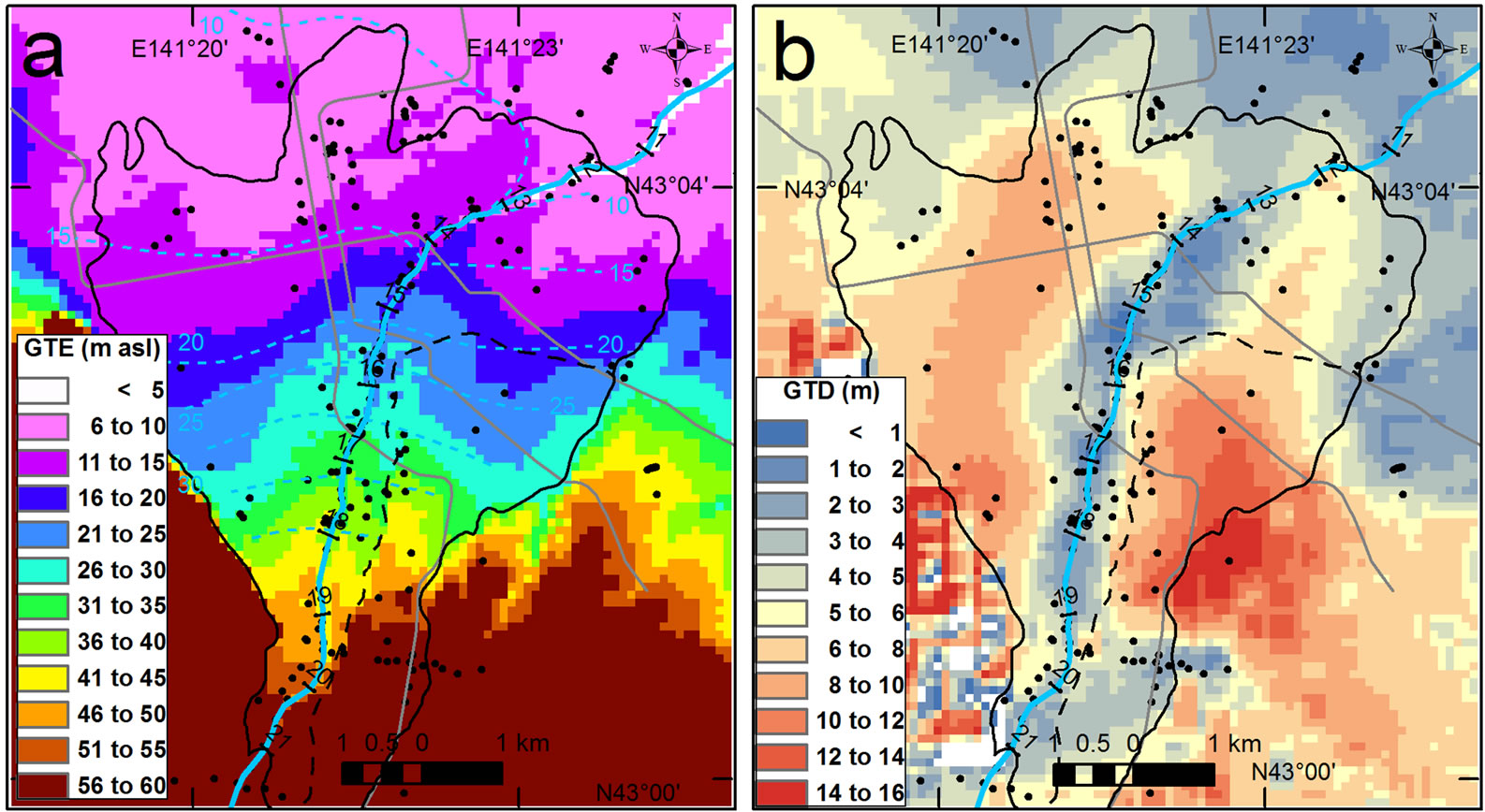
Figure 8. Maps of (a) GTE and (b) GTD in the Toyohira River alluvial fan. Scattered black circles map shallow wells, boreholes, and observation points for river stages. The black solid line denotes the topographic area of the alluvial fan, including the broken boundary line between the Holocene fan and the Pleistocene fan. Short bars along the river denote transects with KP values. The gray lines indicate subway lines through the fan. The broken sky blue lines are water table contours with 5 m intervals (m asl) in April 1960 before subway lines were constructed [25].

Figure 9. (a) VHG map of top screen depths and (b) its variance map in the Toyohira River alluvial fan. Solid circles denote the deep wells used for individual VHG values.

Figure 10. (a) VHG map of middle screen depths and (b) its variance map in the Toyohira River alluvial fan.
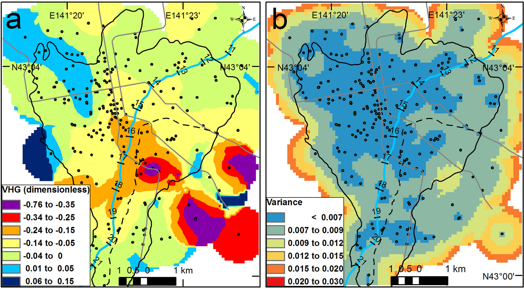
Figure 11. (a) VHG map of bottom screen depths and (b) its variance map in the Toyohira River alluvial fan. The VHG map has proven most valid by cross-validation.
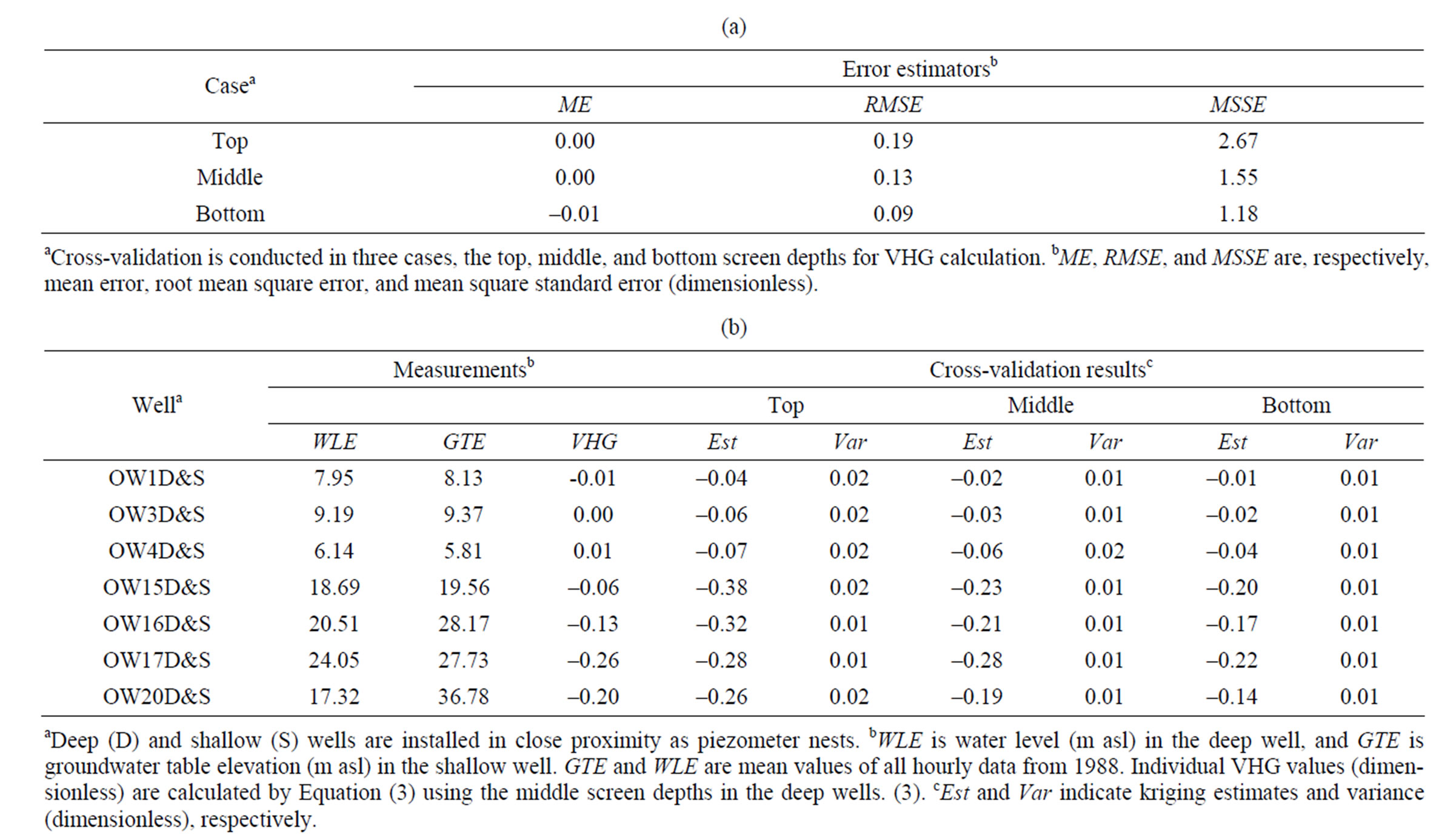
Table 2. Cross validation results for VHG mapping: (a) error estimators and (b) comparison with reliable VHG measurements at piezometer nests.
pears in the Pleistocene fan. The high, steep land surface in the area can be identified as a recharge area. In addition, the water variations (Figure 2) show dewatering by the subway construction in the center of the negative peak (observation well at OW15D and S). Incorporating the recharge and the dewatering probably occurs the negative peak in the Pleistocene fan.
There is also a negative (orange) zone along the river at KP 15.5 - 19. The zone nearly corresponds to the GTE mound and shallow GTD zone, indicating infiltration from the river. The northern (lower) part (KP 15.5 - 17) is in especially good agreement with the distinct losing section found by the synoptic discharge survey [14]. However, the northern peak crosses two subway lines, and heads northwestward along the lines. The dewatering around the subway lines also induces a negative peak of VHG, and increases seepage loss from the riverbed. On the other hand, in the southern (upper) part (KP 17 - 19), the rate of seepage loss is not clearly detected by the synoptic discharge survey. The section corresponds to the sudden depression of the consolidated rock shown in Figure 3. The steep inclination of the basement, in other words, the sudden increase in the thickness of aquifer, probably induces an accumulation of downward groundwater flow at the head. This highlights the potential applicability of the VHG map in obtaining more information about hydrogeologic structure at considerable depth, which is usually accomplished by other geophysical methods such as seismic investigations.
The river discharge observed by synoptic survey was invariable in the southern part (KP 17 - 19), despite the negative VHG peak. The reason remains unrevealed in this study. One argument is that vertical flux of groundwater is small in the section due to large anisotropy of the gravel deposits. Another argument is that net gains and losses are balanced in the section. The GTE map indicates that groundwater might flow through the river from the east (Pleistocene fan) to the west (Holocene fan). In future work, we will quantify groundwater fluxes around the negative peak zone using other approaches such as heat-tracer analysis.
5. Conclusion
Mapping of vertical hydraulic gradient has rarely been attempted on the regional scale because of the lack of piezometer nests and the uncertainty in conventional well data. This study generalized the concept of the traditional plot method, and performed mapping of GTE and VHG by kriging interpolation of conventional well data. The case study site was the Toyohira River alluvial fan, Sapporo, Japan. Water well data from 1988 were divided into those for shallow wells of up to 20 m deep, and deep wells of over 20 m deep. First, the GTE was mapped by adding the topographic drift to the residuals, which were interpolated by ordinary kriging. The drift was formulated as a linear relation between water levels in the shallow wells and the ground surface elevation by ordinary least squares. Next, individual VHG values in the deep wells were calculated by using its top, middle, or bottom elevations of screen depth, respectively. VHG and its variance maps were also generated by using ordinary kriging with a search radius fixed (moving neighborhood kriging). The cross-validation indicated the validity of the GTE map and the VHG map of the bottom screen depths. The other VHG maps of the top and middle screen depths could not be satisfactorily cross-validated. The VHG map, over a wide area, visually reveals the magnitude and extent of recharge and discharge in the fan. The downward flows are predominantly distributed over the fan due to the basement depression at the head, the seepage loss from the river in the middle, and the artificial dewatering in the distal part. The proposed incorporation of VHG and GTE maps provides a quasi- 3D representation, and better insights into 3D groundwater flow fields than do groundwater table maps alone.
6. Acknowledgements
The authors thank the Hokkaido Regional Development Bureau, the administrator of the Toyohira River, for permission to use the observation well data and the hydrologic and hydrogeologic reports for the Toyohira River. We also thank H. Fukami of the Geological Survey of Hokkaido and M. Ishizuka of Aqua Geo Techno, for providing private well data.
REFERENCES
- C. F. Tolman, “Ground Water,” McGraw-Hill, New York, 1937.
- B. R. Rust, “Facies Models 2 Coarse Alluvial Deposits,” In: R. G. Warker, Ed., Facies Models, Geological Association of Canada, Toronto, 1979.
- G. Einsele, “Sedimentary Basins: Evolution, Facies, and Sediment Budget,” Springer, Heidelberg, 2000. doi:10.1007/978-3-662-04029-4
- C. W. Fetter, “Applied Hydrogeology,” Prentice-Hall, Upper Saddle River, 2001.
- S. G. Hu, T. Kobayashi, E. Okuda, A. Oishi, M. Saito, T. Kayaki and S. Miyazaki, “Alluvial Fans-Importance and Relevance: A Review of Studies by Research Group on Hydro-Environments around Alluvial Fans in Japan,” In: M. Taniguchi and I. P. Holman, Eds., Groundwater Response to Changing Climate, CRC Press, AK Leiden, 2010, pp. 131-139. doi:10.1201/b10530-12
- R. A. Freeze and J. A. Cherry, “Groundwater,” PrenticeHall, Englewood Cliffs, 1979.
- C. J. Taylor and W. M. Alley, “Ground-Water-Level Monitoring and the Importance of Long-Term Water-Level Data,” US Geological Survey Circular 1217, US Geological Survey, Denver, 2001.
- W. A. McIlvride and B. M. Rector, “Comparison of Shortand Long-Screen Monitoring Wells in Alluvial Sediments,” Proceedings of the Second National Outdoor Action Conference on Aquifer Restoration, Ground Water Monitoring and Geophysical Methods, Dublin, 1988, pp. 375-390.
- K. R. Rushton, “Groundwater Hydrology Conceptual and Computational Models,” John Wiley & Sons, West Sussex, 2003.
- E. Pardo-Igúzquiza and M. Chica-Olmo, “Estimation of Gradients from Sparse Data by Universal Kriging,” Water Resources Research, Vol. 40, No. 12, 2004. doi:10.1029/2004WR003081
- H. Daimaru, “Holocene Evolution of the Toyohira River Alluvial Fan and Distal Floodplain, Hokkaido, Japan,” Geophysical Review of Japan, Vol. 62A, 1989, pp. 589- 603.
- Y. Sakata, “Geostatistical Reservoir Modeling of Trending Heterogeneity Specified in Focused Recharge Zone: A Case Study of Toyohira River Alluvial Fan, Sapporo, Japan,” PhD Dissertation, Hokkaido University, Sapporo, 2013.
- S. G. Hu, S. Miyajima, D. Nagaoka, K. Koizumi and K. Mukai, “Study on the Relation between Groundwater and Surface Water in Toyohira-Gawa Alluvial Fan, Hokkaido, Japan,” In: M. Taniguchi and I. P. Holman, Eds., Groundwater Response to Changing Climate, CRC Press, AK Leiden, 2010, pp. 141-158. doi:10.1201/b10530-13
- Y. Sakata and R. Ikeda, “Quantification of Longitudinal River Discharge and Leakage in an Alluvial Fan by Synoptic Survey Using Handheld ADV,” Journal of Japan Society of Hydrology and Water Resources, Vol. 25, No. 2, 2012, pp. 89-102. doi:10.3178/jjshwr.25.89
- Y. Sakata and R. Ikeda, “Effectiveness of a High Resolution Model on Groundwater Simulation in an Alluvial Fan,” Geophysical Bulletin of Hokkaido University, Vol. 75, 2012, pp. 73-89.
- L. Nikroo, M. Kompani-Zare, A. R. Sepaskhah and S. R. F. Shamsi, “Groundwater Depth and Elevation Interpolation by Kriging Methods in Mohr Basin of Fars Province in Iran,” Environmental Monitoring and Assessment, Vol. 166, 2010, pp. 387-407. doi:10.1007/s10661-009-1010-x
- N. A. C. Cressie, “Statistics for Spatial Data,” John Wiley & Sons, New York, 1993.
- T. Hengl, “A Practical Guide to Geostatistical Mapping of Environmental Variables,” JRC Scientific and Technical Reports, Office for Official Publications of the European Communities, Luxembourg, 2007.
- P. K. Kitanidis, “Generalized Covariance Functions in Estimation,” Mathematical Geology, Vol. 25, No. 5, 1993, pp. 525-540. doi:10.1007/BF00890244
- B. Minasny and A. B. McBratney, “Spatial Prediction of Soil Properties Using EBLUP with the Matérn Covariance Function,” Geoderma, Vol. 140, No. 4, 2007, pp. 324-336. doi:10.1016/j.geoderma.2007.04.028
- G. de Marsily, “Quantitative Hydrogeology,” Academic Press, Orlando, 1986.
- P. Goovaerts, “Geostatistics for Natural Resources Evaluation,” Oxford University Press, New York, 1997.
- H. Wackernagel, “Multivariate Geostatistics: An Introduction with Application,” Springer, Berlin, 2003. doi:10.1007/978-3-662-05294-5
- J. P. Chilès and P. Delfiner, “Geostatistics Modeling Spatial Uncertainty,” John Wiley & Sons, New York, 1999. doi:10.1002/9780470316993
- H. Yamaguchi, “Water Quality in Sapporo City,” In: Board of Education of Sapporo City, Ed., Water in Sapporo City, Hokkaido Shimbun Press, Sapporo, 1983.
- H. Osanai, K. Matsushita and H. Yamaguchi, “Geological Map of Hokkaido No. 1 Sapporo,” Geological Survey of Hokkaido, Sapporo, 1974.
NOTES
*Corresponding author.