Journal of Water Resource and Protection
Vol. 2 No. 8 (2010) , Article ID: 2457 , 9 pages DOI:10.4236/jwarp.2010.28086
Comparison of Discharge Duration Curves from Two Adjacent Forested Catchments—Effect of Forest Age and Dominant Tree Species
Forestry & Forest Products Research Institute, Tsukuba, Japan
E-mail: a123@ffpri.affrc.go.jp
Received May 20, 2010; revised June 18, 2010; accepted June 30, 2010
Keywords: Paired-Watershed Experiment, Forest Age Difference
ABSTRACT
The effects of forest age and dominant tree species on the water discharge volume have been analyzed by a paired-watershed experiment in two adjacent catchments in Tatsunokuchi-yama Experimental Forest, western Japan. The control period is 1937-1943. The treated periods are 1948-1953, 1968-1977, and 1996-2003. In these treated periods, the forest age or the dominant tree species were different between two adjacent periods. Differences in the discharge duration curves from the two catchments are compared for the control and the treated periods. A significant change in the discharge duration curves is seen in the third treated period (1996-2003) on days with low water, when the forest age difference between the adjacent catchments was 35 years. This is believed to be the result of differences in forest age and forest treatment just after the occurrence of pine wilt disease.
1. Introduction
In recent years, the expectation for the various functions of forests has become wide spread. These functions include those relating to the forest’s water budget, such as water resource management and flood prevention. What forest type performs best in terms of these functions is of major interest in forest hydrology. First, two typical indicators can be given for classifying forest types: tree species and stand age.
Bosch and Hewlett [1] compared water budgets in broad-leaved and coniferous forest catchments, and found that deciduous forests perform better in terms of water resource management. This was rebutted by Tanaka and Suzuki [2]. Moreover, some studies have used mathematical modeling techniques to examine forest type and water budget, e.g., the reviews conducted by Komatsu [3] and Komatsu et al. [4].
On the other hand, Kuczera [5] provided a curve to show the relationship between forest age (extending up to 200 years) and annual water discharge volume for forest catchments in Australia dominated by eucalyptus and ash. Also, Kosugi and Katsuyama [6] reported change over time in evapotranspiration in Japanese cypress stands. However, there have been few studies of the relationship between stand age and water discharge.
Tatsunokuchi-yama Experimental Forest, located in western Japan, has two very similar adjacent forested catchments. The forest in one catchment has been dominated by deciduous broad-leaved species since 1947, and it has existed without disturbances. The forest in the other catchment has a history of forest fires and the occurrence of pine wilt disease. This catchment’s species has varied with time between broad-leaved and coniferous trees. Thus, these two catchments areas have forest features that are significantly different. The effects of forest age and dominant tree species on the water discharge volume has been analyzed and reported in this paper by comparing the discharge volumes during each of the three periods as the differences in forest features in the two catchments have changed with time.
2. Method
2.1. Experimental Forest
The Tatsunokuchi-yama Experimental Forest is located at 34°42’ N, 133°58’ E (Figure 1). Annual precipitation and mean air temperature are approximately 1200 mm
 (a)
(a)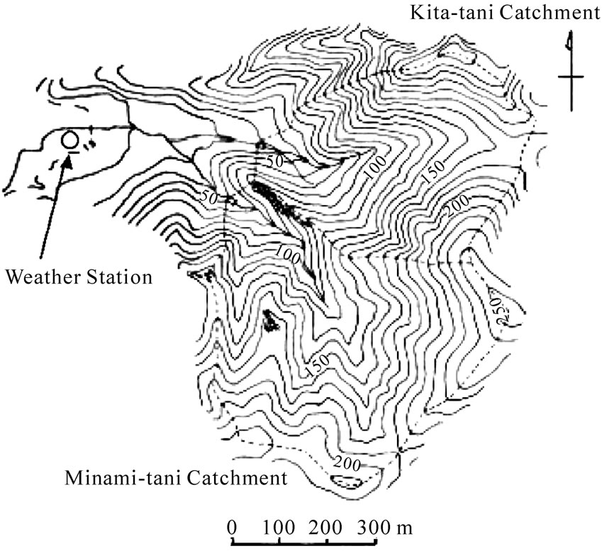 (b)
(b)
Figure 1. Location (a) and topography (b) of Tatsunokuchi-yama Experimental Forest.
and 14.3°C, respectively. The seasonal distribution of precipitation shows little precipitation and almost no snow in the winter, while precipitation is heavy in the months of June, July, and September because of the effects of the rainy season and hurricanes. Precipitation is low compared to other locations in Japan, and the soil can enter a markedly dry state in the summer. Geologically, the area is part of the Chichibu Paleozoic strata, and the soil is a clay soil with significant admixture of gravel classified as a clay loam. The adjacent two catchments are Kitadani (KT, 17.3 ha) and Minamidani (MN, 22.6 ha), and are mainly underlain by Paleozoic formations. Discharge and precipitation have been measured at or near the site since 1937; discharge was measured in the forest using a wire gauge, and precipitation was measured at an adjacent weather station using a rain gauge.
2.2. Forest History
An overview of forest history in the test area is shown in Table 1. The Tatsunokuchi-yama Experimental Forest was established in 1937 to conduct paired-watershed experiments. Red pine (Pinus densiflora) was the dominant species at the site in 1937. However, the forest began declining in 1940 as a result of pine wilt disease, and timber was harvested in all areas of the KT and MN watersheds in 1944-1947 and 1944-1945, respectively. Natural regrowth of red pine, oak (Quercus serrata), and bamboo (Pleioblastus chino) occurred in both watersheds. Deciduous broad-leaved trees have since dominated KT, but the vegetation in MN has been repeatedly disturbed over the years.
In 1954-1957, brush cutting was done over 19.5 ha in the MN catchment. In 1959, 22.3 ha of forest were lost because of forest fire. The burnt area was planted with Japanese black pine in 1960, but in 1978-1980, the black pines were completely destroyed by pine wilt disease. After that, the area was left to recover naturally, and the natural growth consisted primarily of broad-leaved trees.
Changes in stand volume since 1958 are shown in Table 2.
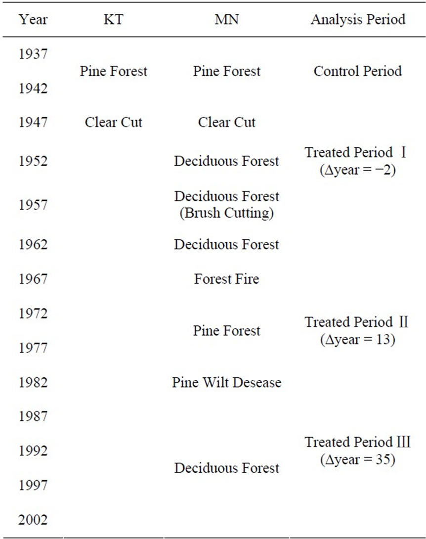
Table 1. Vegetation history in KT and MN catchments and analysis period definition.

Table 2. Historical record of stand volume in Tatsunokuchi-yama Experimental Forest.
Many studies have been conducted in the Tatsunokuchi-yama Experimental Forest. Fujieda et al. [7] and Abe and Tani [8] compared the annual discharge volumes from KT and MN. They found MN to have the larger discharge volumes in 1960-1967 and 1981-1996, just after the disturbances by forest fire and pine wilt disease, respectively. In contrast, KT had larger annual discharge volumes than MN in other periods when forest canopy is closed in both catchments. An increase in discharge after periods of forest fires and pine wilt disease has been reported in Fujieda et al. [7], Abe and Tani [8] and Tamai et al. [9].
2.3. Paired-Watershed Experiment
In KT, forest growth has been consistent since 1948. In MN, on the other hand, the forest was partially lost because of forest fire in 1960 and pine wilt disease in 1978-1980. Therefore, the value obtained by subtracting the MN forest age from the KT forest age (∆year) varied from −2 years to 13 years to 35 years (Table 1). One purpose of this study is to evaluate the effects of forest age on the discharge duration curve using a paired-watershed experiment to compare changes due to ∆year in the relative relationship of the discharge duration curves for KT and MN. KT is taken to be the control catchment (undisturbed), and MN the treated catchment.
Factors affecting the discharge duration curve are classified into three main types: 1) precipitation pattern, 2) vegetation, and 3) territorial functions such as topography and geology. In a paired-watershed experiment, it is possible to cancel out differences in precipitation pattern by comparing the discharge duration curves from two adjacent catchments [1]. If the forests of both catchments are in the same state during the control period, then the effects of vegetation are canceled out. Therefore, the relative relationship of the discharge duration curves in the control period is regarded as being attributable to differences in territorial functions.
Differences arose in the forests of the two catchments during the treated periods. Therefore, the relative relationship of the discharge duration curves from the two catchments differed from their relative relationship in the control period. By evaluating changes in the relative relationship in the control period and treated periods, it is possible to clarify the effects of the forest differences arising during the treated periods on the discharge duration curves.
In this research, the control period is from 1937, when the experimental forest was established, to 1943, the year before timber harvesting began in both catchments. There were some differences in forest vegetation between the two areas in 1937. In KT, one part (~5 ha) was grass in a previously harvested area, and the rest was natural stands of old/middle-growth red pine. In MN, there were new-growth stands (~6 ha) and old/middle-growth stands (~10 ha) of natural red pine, and a very small area (~1 ha) of planted Japanese cypress stands. However, the stand age of the main stands of old/middle-growth red pine was sufficiently large, so that the difference in stand age can be regarded as non-existent compared to the treated periods described below.
Timber harvesting ended in 1947 in KT and 1945 in MN. Consequently, ∆year from 1948 until 1958, the year before the wildfire, is −2. Incidentally, Tamai [10] has reported that brush cutting was conducted over 19.5 ha in 1954-1957, and effects of this on the discharge duration curve are significant in that period. Therefore, the period 1948-1953, excluding the period after 1954, is taken to be treated period I with a ∆year of −2.
In 1960, Japanese black pine was planted in the part of MN burnt by forest fire. Therefore, ∆year is 13 for the period from 1960 to 1977, the year before the pine wilt disease occurred. Fujieda et al. [7] and Tamai et al. [9] have evaluated the effects of forest loss in the period 1960–1964, taking that as the period affected by forest fire. Hence, the subsequent period, 1965-1977, was taken to be treated period II with a ∆year of 13. However, since daily discharge was not observed for some days in 1967 and 1974, those years were excluded from the analysis.
Vegetation in the area of MN where the black pines were completely destroyed in 1980 was left to recover naturally as a deciduous broad-leaved forest. Therefore, the ∆year after 1981 is 35. Abe and Tani [8] and Tamai et al. [9] have evaluated the effects of forest loss in the period 1981-1984, taking that as the period affected by pine wilt disease. On the other hand, there was a disturbance in 2004 where about 1.7 ha of forest in MN was lost due to wind-toppling. Thus, the period 1996-2003 is taken to be treated period III with a ∆year of 13. However, since daily discharge was not observed for some days in 1997, those years were excluded from the analysis.
Values for daily discharge in KT and MN were obtained from Forest Experiment Station Ministry of Agriculture and Forestry [11], Forest Influence Unit and Okayama Experimental Site [12], Forest Influence Unit and Okayama Experimental Site [13], Goto et al. [14] and Tamai et al. [15].
2.4. Discharge Duration Curves
In a discharge duration curve, the 365 daily discharges for one year are arranged in descending order. The left side of the curve indicates daily discharges at times of high water, and the right side indicates daily discharges at times of low water.
The discharge duration curves for KT and MN are compared. A linear regression with a high correlation (Equation (1)) can be obtained between the two catchments in the control period.
Qm (year, i) = ai Qk (year, i) + bi(1)
Here Q* (year, i) indicates the discharge volume (mm day−1) for the ith day of the discharge duration curve for the given year, and ai and bi indicate the slope and intercept, respectively, of the linear regression.
Qmcal (year, i) is calculated using Equation (2) by substituting the observed discharge volume from KT in the treated period (Qkobs(year, i)) into Equation (1) obtained for the control period, and can be regarded as an estimated value for the discharge volume from MN expected when the forests in both catchments were in the same state (i.e., had the same forest age and tree species in this study).
Qmcal (year, i) = ai Qkobs (year, i) + bi (2)
∆Qm (year, i) is calculated with Equation (3) and indicates the change in discharge volume because of the difference in the forest states of MN and KT, in terms of age or tree species.
∆Qm (year, i) = Qmobs (year, i) – Qmcal (year, i) (3)
Here Qmobs (year, i) indicates the observed discharge volume from MN during the treated period.
If the water year is taken from April until March of the following year in the Tatsunokuchi-yama Experimental Forest, then there is only one dry season in one water year, and correlation between the discharge volumes from both catchments increases [16]. Therefore, this study takes one water year from April to May of the following year. For example, the discharge duration curve indicated by year = 1997 is for the period from April 1997 to March 1998.
3. Results
3.1. Relative Relationship of Discharge Duration Curves from KT and MN during the Control Period
Figure 2 shows ai, bi, and the correlation coefficient of the regression line found for Equation (1) for the control period. The value b1 = −2.5518 was extremely small compared to other values and could not be shown in Figure 2(a). The correlation coefficients for i = 3 and 26 were extremely small (0.9418 and 0.9479, respectively), but correlation coefficients for all other days were 0.95 or higher, and thus the correlation is sufficient for estimating Qmcal (year, i) using Equation (2).
Figure 3 shows curves that average the respective discharge duration curves from MN and KT over the 7 years of the control period. The difference between the two is not clear, but the discharge duration curve for MN is located just slightly above that for KT. The difference is clearly observable in the range i = 100 – 200. This difference is caused by the difference in territorial functions such as topography and geology.
 (a)
(a)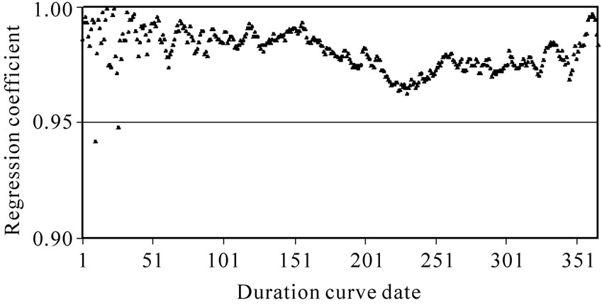 (b)
(b)
Figure 2. Regression lines between daily discharge volume in discharge duration cuves from KT and MN catchments during control period. (a) Regression coefficient (dark point with left-axis) and regression constant (black point with right axis). The regression constants at i = 1, 2 and 3 are out of range in this figure to be –2.5518, -0.6036 and –0.6329, respectively; (b) Correlation coefficient.
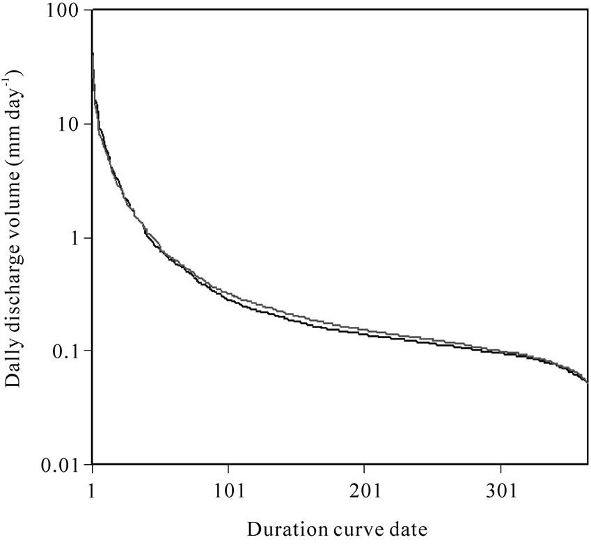
Figure 3. Averaged discharge duration curves during control period. Black line; KT. Gray line; MN.
3.2. Differences in Discharge Duration Curves in Each Treated Period
Figure 4 shows the relationship between Equation (2), and Qkobs (year, i) and Qmobs (year, i) in the control period and treated period for i = 3, 35, 95, 185, 275, and 355. The X-axis indicates Qkobs (year, i) and the Y-axis indicates Qmobs (year, i). Of the three lines, the thick line in the center indicates Equation (2), and the thin lines on both sides indicate the range of the significance level at 90%. If white points are plotted to the upper left side on the regression line, it indicates that the daily discharge volume from MN increases because of the difference between the forested states in both catchments; if those points are plotted to the lower right, it indicates that the daily discharge volume from MN decreases. When white points are plotted far away from the regression line, it indicates that the change in the daily discharge volume from MN is large and the effect is significant. This is caused by the difference in the forest age and dominant species. In other words, white points plotted to the outside of the thin lines indicate that the change compared to the control period is significant at a significance level of 90%.
As a general trend, there are a few points plotted to the lower right of the graph, when i is in the 3–95 range. When i is in the 185–355 range, however, the number of points plotted to the upper left of the graph increases. This means that the relative relationship of Qkobs (year, i) and Qmobs (year, i) in the control period and treated periods varies depending on the size of the daily discharge volume.
It is possible to determine a hypothetical discharge duration curve from MN in each year of the treated period on the basis of the value of Qmcal (year, i) calculated using Equation (2). This is the potential discharge duration curve that would likely have been obtained if the MN forest had the state as KT, without losses due to forest fire in 1959 and pine wilt disease in 1978–1980. Figure 5 shows the average of the potential discharge duration curves for each of the treated periods I, II, and III, together with the actual observed discharge duration curves. The area between the two discharge duration curves indicates the change in the curves that is thought to have occurred because the stand state is different between MN and KT. Although it is not shown in Figure 5, the relationship between the potential discharge duration curve for MN and the observed discharge duration curve for KT is the same as that between the discharge duration curves observed for MN and KT in the control period shown in Figure 3. In other words, the discharge duration curve observed for KT is located slightly below the potential MN curve. Therefore, the difference in the curves, which is thought to be due to the different forest state in the MN and KT catchments, becomes somewhat smaller than the difference in the actual observed curves of the two catchments.
The difference between the two discharge duration curves shown in Figure 5 is not clearly significant for treated period I. For treated period II, the difference is barely significant in the range i > 300. For treated period III, on the other hand, the difference is clearly significant in the range i > 100. However, the vertical axes in Figure 5 are on a logarithmic scale, and thus it is difficult to see any difference in the range where i is small. Therefore, the average values of ∆Qm (year, i) for i = 3, 35, 95, 185, 275, and 355 are shown in Table 3. A positive value indicates that the discharge volume from MN is calculated to increase because of the difference in forest state between MN and KT. Overall, ∆Qm (year, i) exhibits a tendency to increase as ∆year and i increase. However, the values found in this study are extremely small compared to ∆Qm (year, i) in cases where the forest was destroyed by forest fire or pine wilt disease. Exceptions to this are i = 275 and 355 in treated period III.
Figure 6 shows the changes in the ratio (percentage) obtained by dividing the values of the discharge duration curve observed for MN by the values of the hypothetical discharge duration curve (Qmobs (year, i)/Qmcal (year, i)). When this value is above 100%, it means that the discharge has increased because of the difference in forest state between MN and KT, and conversely, when the value is below 100%, it means that the discharge has decreased for the same reason. Qmobs (year, i)/Qmcal (year, i) tended to increase as ∆year increased. In terms of the range of i, where Qmobs (year, i)/Qmcal (year, i) exceeds 100%, there is a gradually increasing number of days exceeding 100%—none for treated period I, i > 169 for treated period II, and i > 50 for treated period III. However, except for treated period III, the value of Qmobs (year, i)


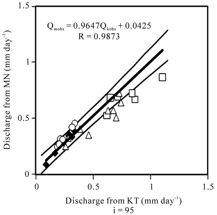
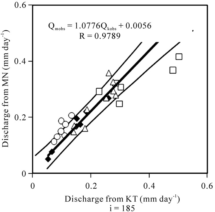
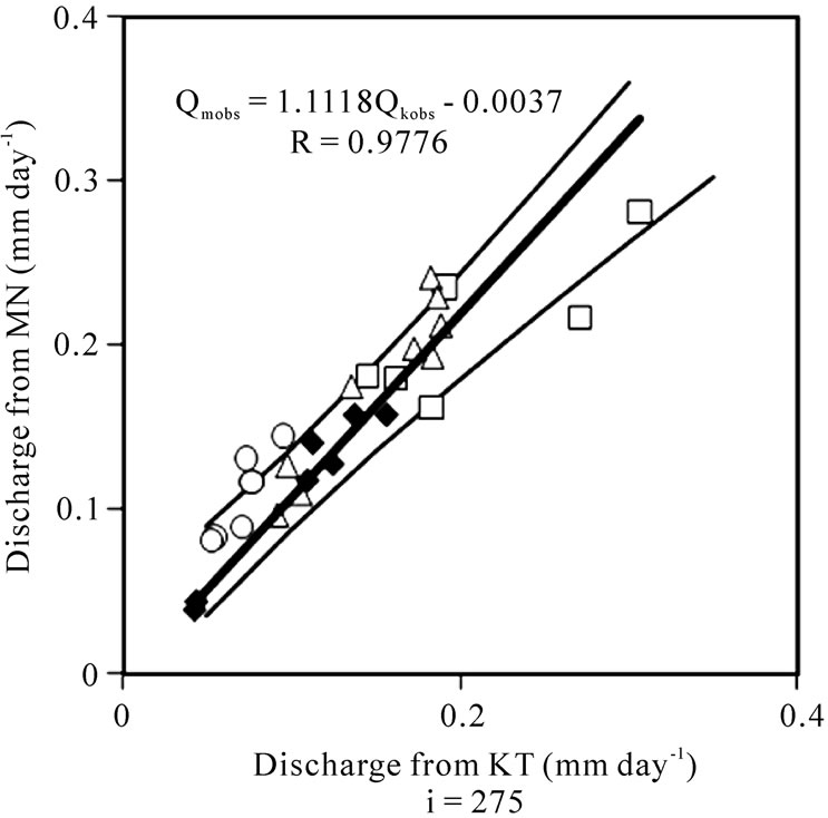
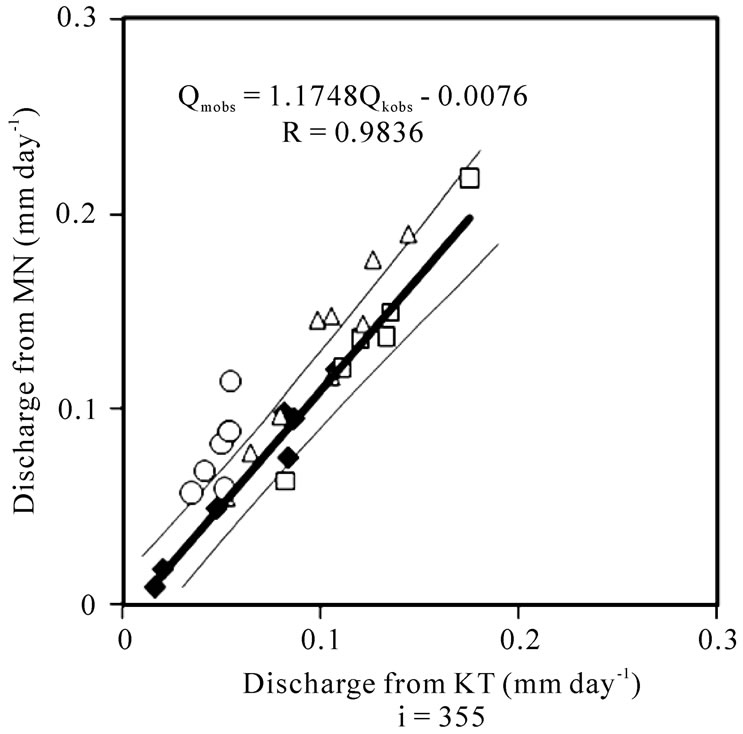
Figure 4. Relationships between observed daily discharge volumes from KT and MN. Black diamond; Control period, White square; Treated period I, White triangle; Treated period II, White circle; Treated period III, Thick line; Regression line in control period, Thin lines; Significant range at 90% reliability.
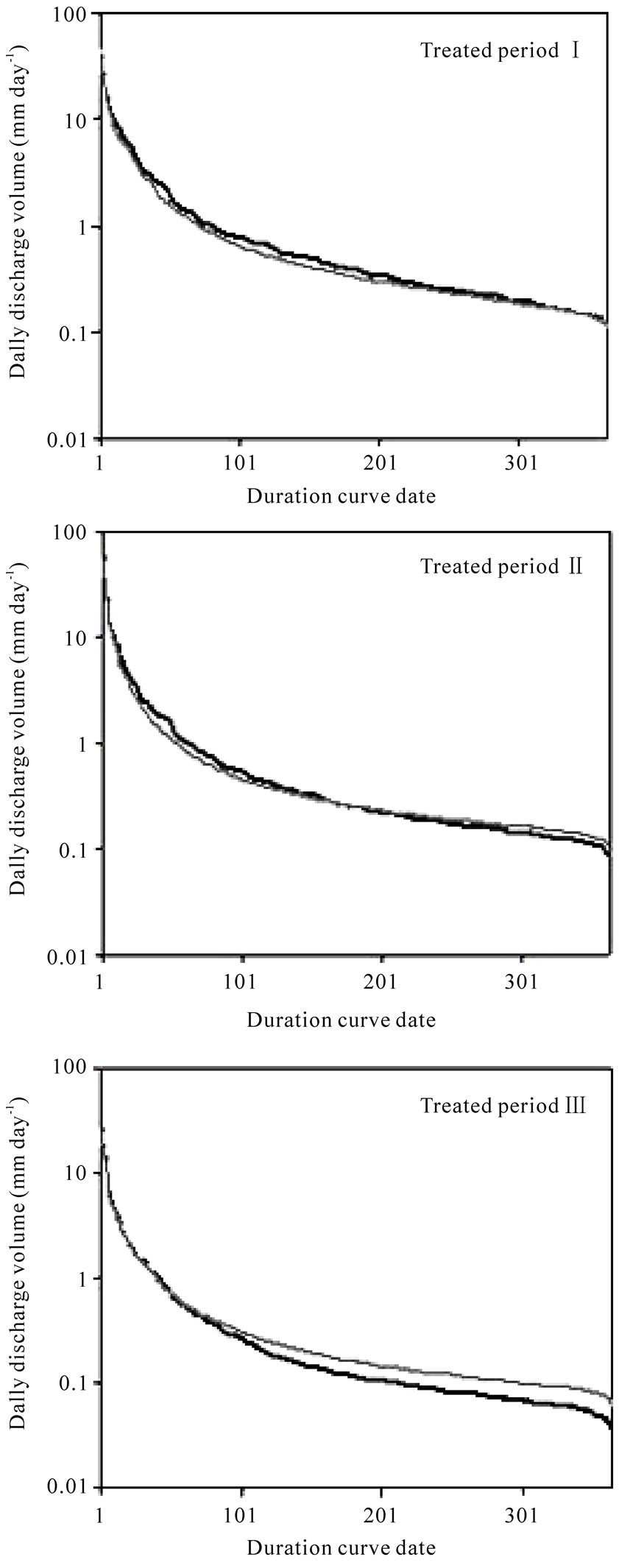
Figure 5. Increased averaged discharge duration curves in each treated periods caused by younger forest age or forest disturbances. Gray line; Observed duration curve from MN. Black line; Calculated duration curve from MN This line is also regarded as the potential curves from MN when same Equation (1) would be adaptable even in the treated periods.
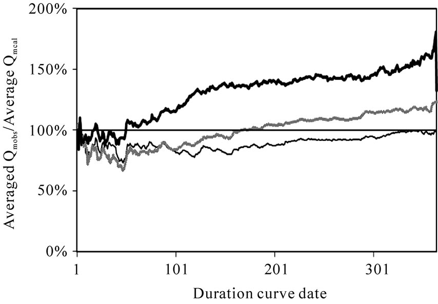
Figure 6. Estimated increased ratio of daily discharge compared with the control period caused by younger forest age or forest disturbances. Thin black line; Treated period I, Gray line; Treated period II, Thick black line; Treated period III.
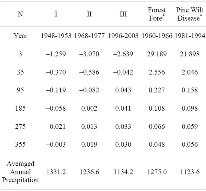
Table 3. Estimated increased volume from MN compared with the control period caused by younger forest age or forest disturbances.
/Qmcal (year, i) is close to 100%. That is, the change was small. In the range of i > 307 for treated period III, the value of Qmobs (year, i)/Qmcal (year, i) became larger than 150%. This means that the discharge volume from MN during the about 60 days of low water was about 1.5 times greater than the reference. The value of Qmcal (year, i), used as the reference, is the discharge volume from MN expected if the forest was the same as KT, and had not been destroyed due to events such as forest fire and pine wilt disease. Therefore, if the value of Qmcal (year, i) is taken to be the standard, then there are about 60 days of low water. However, since discharge volume in the time of low water has a smaller absolute volume, there is little change in the annual discharge volume. In terms of the average value for treated period III, Qmobs (year, i) was 229.832 mm year−1, but ∆Qm (year, i) was only 1.402 mm year−1.
4. Discussion
Discharge volume from MN is calculated to be 1.5 times greater during the about 60 days of low water in treated period III. There are three possible reasons: 1) The effect of the forest loss because of pine wilt disease has continued in treated period III because the vegetation was left to recover naturally. 2) The forest age in KT is larger in treated period III than other periods. Thus, the large ∆year causes the large difference between the discharge volumes from KT and MN. 3) In treated periods I and III, the dominant species in MN was deciduous broad-leaved trees, the same as in KT. However, in treated period II, it was coniferous evergreen trees, different from that in KT. The difference in the dominant species might cause the difference in discharge volumes between the catchments. On the basis of this hypothesis, ∆Qm (year, i) in treated period II would be as large as in treated period III. The three possibilities are discussed below.
4.1. Vegetation Treatment Differences after Disturbances
In the case of treated period II, Japanese black pine was planted in the damaged area in MN in 1960 just after the forest fire. It took five years for the discharge volume from MN to recover from the effects of the forest fire [7]. On the other hand, in the case of treated period III, the vegetation was left to recover naturally after the pine wilt damage. It took 16 years for the annual discharge volume from MN to recover to almost the same discharge volume as KT. However, the low (i = 265) and drought (i = 355) discharges had not recovered even by 2004 [10]. The difference in how the vegetation was treated after the loss of the forest may have caused the difference in the discharge volume between treated period III and the other treated periods.
4.2. Differences in Forest Age
If the large value of ∆year causes the large difference between the discharge volumes from both catchments, this suggests that the water loss effect of the old forest in KT has changed from that when it was younger. Kuczera [5] found the relationship between the forest age and annual discharge volume for forest catchments in Australia that were dominated by eucalyptus and ash, and proposed a curve where water discharge reaches a minimum with a forest age of 25 years and increases after that. A decrease of 50-400 mm year−1 was found at a forest age of 25 years. On the other hand, Kosugi and Katsuyama [6] found seasonal changes in evapotranspiration of a Japanese cypress forest using the short-term water discharge method, and there were no clear differences, in terms of seasonal fluctuations or yearly volume, over a period of 33 years.
In this study, it was calculated that for about 60 days at the time of low water, discharge from KT with an age of 49-56 years was reduced to 2/3 or less of the discharge from MN with an age of 16-23 years in treated period III. In the forest age relationship in the Kuczera curve [5], discharge from a 49-56 year old forest catchment was larger than that from a 16-23 year old forest catchment. This difference may be because the forest growth rates in the KT and MN catchments are smaller than those in the forests studied by [5], and the forest age exhibiting the minimum value is larger.
Vertessy et al. [17] reported that the Sapflow area index (SAI) or Leaf area index (LAI) decrease is the cause of the discharge increase from a forest catchment with the age of 25 year or older. Goto et al. [18] reported the LAI in the KT catchment increased from 7.0 in 1998 to 8.0 in 2005. This LAI increase was concurrent with the increase in forest age in KT, from 50 in 1998 to 57 in 2005. Thus, the evaporation rate is supposed to increase with forest age. Also, in the Kuczera curve, there is a reduction of 50-400 mm year−1 when the forest age is 25 years. However, the increase in this study was only 1.402 mm year−1, and thus no large change was seen. This agrees with the results of [6].
The forest in KT grew even when the forest age was 50-57. Thus, the maturity might cause the low and drought discharge volume from KT to be larger than that from MN in treated period III.
4.3. Differences in the Dominant Species
The dominant tree species of MN in treated period II was Japanese black pine, which is different from KT. Therefore, in addition to differences in forest age, there is a possibility that effects due to differences in dominant tree species are also included in ∆Qm (year, i) for treated period II. [4] conducted model calculations of annual evapotranspiration of three catchments, including MN in 1971-1977 and 1996-2000, and found that evapotranspiration of broad-leaved trees was almost equal to that of young coniferous forests. The forest age in MN in treated period II was young (8-18 years). Therefore, it is thought that differences in dominant tree species had little effect on ∆Qm (year, i) in treated period II. Similarly, the difference in the dominant species in MN between periods II and III had little effect on the large volume of ∆Qm (year, i) in treated period III.
5. Conclusions
In this study, we found that discharge for about 60 days in the time of low water from KT in treated period III was reduced to 2/3 or less of that from MN of Tatsunokuchi-yama Experimental Forest, Okayama City. Possible causes are 1) vegetation treatment differences after disturbances, 2) differences in forest age, and 3) differences in the dominant species. This study concluded that 3) cannot be the cause. However, 1) and 2) are possible causes. Both are related to forest management practices. This means that periodic and adequate forest treatment is necessary to maintain water discharge at low water events. However, since this study was limited to two catchments and limited samples, it will be necessary to further these studies using an increased number of sampling periods and catchments.
REFERENCES
- J. M. Bosch and J. D. Hewlett, “A Review of Catchment Experiments to Determine the Effect of Vegetation Changes on Water Yield and Evapotranspiration,” Journal of Hydrology, Vol. 55, No. 1, 1982, pp. 3-23.
- T. Tanaka and K. Suzuki, “Reconsideration on the Histrical Papers Reporting the Effect of Vegetation Changes on Water Yield,” Water Science, Vol. 52, No. 300, 2008, pp. 46-68.
- H. Komatsu, “Forest Categorization According to DryCanopy Evaporation Rates in the Growing Season: Comparison of the Priestley-Taylor Coefficient Values from Various Observation Sites,” Hydrological Processes, Vol. 19, No. 19, 2005, pp. 3873-3896.
- H. Komatsu, N. Tanaka and T. Kume, “Do Coniferous Forests Evaporate More Water than Broad-Leaved Forests in Japan?” Journal of Hydrology, Vol. 336, No. 3-4, 2007, pp. 361-375.
- G. Kuczera, “Prediction of Water Yield Reductions Following a Bushfire in Ash-Mixed Species Eucalypt Forest,” Journal of Hydrology, Vol. 94, No. 21, 1987, pp. 215-236.
- Y. Kosugi and M. Katsuyama, “Evapotranspiration over a Japanese Cypress Forest. II. Comparison of the Eddy Covariance and Water Budget Methods,” Journal of Hydrology, Vol. 334, No. 3-4, 2007, pp. 305-311.
- M. Fujieda, T. Kishioka and T. Abe, “Effects of Forest Fire on Runoff from Minami-Tani, Tatsunokuchi-Yama,” Journal of Japanese Forest Society, Vol. 61, No. 5, 1979, pp. 184-186.
- T. Abe and M. Tani, “Streamflow Changes after Killing of Pine Trees by the Pine-Wood Nematode,” Journal of Japanese Forestry Society, Vol. 67, No. 7, 1985, pp. 261-270.
- K. Tamai, Y. Goto, T. Miyama and Y. Kominami, “Influence of Forest Decline by Forest Fire and Pine Wilt Disease on Discharge and Discharge Duration Curve: In the Case of Tatsunokuchi-Yama Experimental Forest,” Journal of Japanese Forest Society, Vol. 86, No. 4, 2004, pp. 375-379.
- K. Tamai, “A Paired-Catchment Experiment in the Tatsunokuchi-Yama Experimental Forest, Japan: The Influence of Forest Disturbance on Water Discharge,” WIT Transactions on Ecology and Environment, Vol. 83, 2005, pp. 173-181.
- Forest Experiment Station Ministry of Agriculture and Forestry, “Statistical Report of Hydrological Observation at Experimental Watersheds (Daily Discharge Volume and Precipitation),” Forest Experiment Station in Ministry of Agriculture and Forestry, 1961, p. 255.
- Forest Influences Unit and Okayama Experimental Site, “Statistical Report of Hydrological Observation at Tatsunokuchiyama Experimental Watershed,” Annual report of Kansai Branch Station, Forest Experiment Station, No. 22, 1981, pp. 56-62.
- Forest Influences Unit and Okayama Experimental Site, “Statistical Report of Hydrological Observation at Tatsunokuchiyama Experimental Watershed (January, 1959- December, 1977),” Bulletin of Forestry & Forest Products Research Institute, No. 308, 1979, pp. 133-195.
- Y. Goto, K. Tamai, Y. Kominami and T. Miyama, “Hydrological Observation Reports in Tatsunokuchi-Yama Experimental Forest (January, 1981-December, 2000),” Bulletin of Forestry & Forest Products Research Institute, Vol. 4, No. 1, 2005, pp. 87-133.
- K. Tamai, Y. Goto, Y. Kominami, T. Miyama and I. Hosoda, “Hydrological Observation Reports in Tatsunokuchi-Yama Experimental Forest (January, 2001-December, 2005),” Bulletin of Forestry & Forest Products Research Institute, Vol. 7, No. 3, 2008, pp. 125-138.
- N. Inaba, K. Kondo, S. Numamoto and S. Hayashi, “Influence of the Definition of Water-Year Period on Discharge Duration Analysis Forcused on Low Flow: In the Case of the Tatsunokuchi-Yama Experimental Watershed,” Journal of Japanese Forest Society, Vol. 89, No. 6, 2007, pp. 412-415.
- R. A. Vertessy, F. G. R. Watson and S. K. O’Sullivan, “Factors Determining Relations between Stand Age and Catchment Water Balance in Mountaion Ash Forests,” Forest and Ecology Management, Vol. 143, No. 1, 2001, pp. 13-26.
- Y. Goto, K. Tamai, T. Miyama, Y. Kominami and I. Hosoda, “Effects of Disturbance on Vertical Stratification of Broad-Leaved Secondary Forests in Tatsunokuchi-Yama Experimental Forest,” Bulletin of Forestry & Forest Products Research Institute, Vol. 5, No. 3, 2006, pp. 215- 225.
- M. Fujieda and T. Abe, “Afforestation on Streamflow on Tatsunokuchiyama Experimental Watershed,” Bulletin of Forestry & Forest Products Research Institute, No. 317, 1982, pp. 113-138.