ABSTRACT

In this article an M/G/1 queueing model with single server, Poisson input, k-phases of heterogeneous services and Bernoulli feedback design has been considered. For this model, we derive the steady-state probability generating function (PGF) of queue size at the random epoch and at the service completion epoch. Then, we derive the Laplace-Stieltjes Transform (LST) of the distribution of response time, the means of response time, number of customers in the system and busy period.

1. Introduction

The M/G/1 queueing model is one of the famous and applied models in which the distribution of service times is unknown. For this reason, many of real models could be considered by this model. Multi-phase service is important, because some of systems have more than one phase service, for example manufacture production lines. Feedback is also important, because in some queueing models, some customers, after completion the service, may need to go back to the end of queue to take the service again. It means that the service customer is not acceptable and must go to the end of queue. According to these conditions, we have considered an M/G/1 queueing model with k-Phase Optional Services and Bernoulli feedback.

For this model, first we find the steady-state probability generating function (PGF) of queue size at the random epoch and at the service completion epoch. Then, we derive the Laplace-Stieltjes Transform (LST) of the distribution of response time. The means of response time, number of customers in the system and busy period will be derived by using the PGF and LST.

In relation of this model, [1-9,11] have derived some results. The model that they have considered is two phases. But, in this article, we will consider a k-phase queue with optional service and Bernoulli feedback in all phases. Of course, [10] studied an M/G/1 queue with k-phase services and vacation, but without feedback that is different from this paper.

Following, in section 2 we describe the model and give some definitions. In section 3, the PGF of the system size will be derived. In section 4, we will find some measures of effectiveness. At the final section, we provide a conclusion.

2. The Mathematical Model and Definitions

In this model, the server provides first phase of regular service to all the customers. As soon as the i-th (for i = 1, ∙∙∙, k − 1) phase of service of a customer is completed , it may leave the system or immediately go for (i + 1)-th phase of optional service. However, after receiving each phase of unsuccessful service by a unit, then it may immediately join to the end of tail of the original queue as feedback customer to take service again. Thus, the assumptions of the model are:

1) Customers arrive at the system to a Poisson process with rate.

2) The service discipline of the system is FCFS1.

3) The server provides k-phases of heterogeneous service for any customer. The service times for k-phases are independent random variable that denoted by with distribution functions and LST of these distributions are. These variables have finite moments, that is for.

4) As soon as the i-th phase of service of a customer is completed, the customer may go to the (i + 1)-th phase of service with probability.

5) After completion of the i-th phase, if the customer is dissatisfied with its service for certain reason or it received unsuccessful service, in this case the customer may immediately joins the end of the original queue as a feedback customer for receiving the service again with probability, for, otherwise the customer may depart the system with probability.

Definition 2.1. The modified service time or the time required by a customer to complete the service cycle is given by

(2.1)

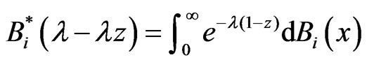
where and. Then the LST of B is given by

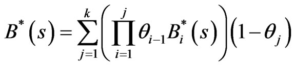(2.2)

and

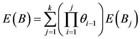(2.3)

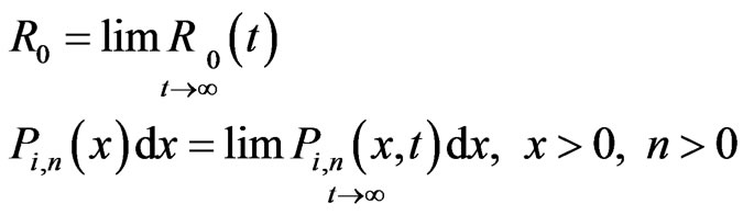
As we know, in the queueing systems the utilization factor is and denoted by. This measure says if the system is in steady state or not. In this article, we study the model in equiblirium. It happens when.

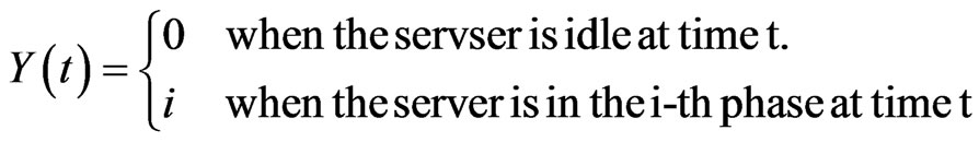
Definition 2.2. The elapsed of i-th phases service at time “t” is denoted by for. We introduce the random variable as follow

Thus, we have a bivariate Markov process 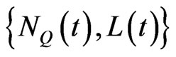, where if and if, for. Now, we define probabilities as

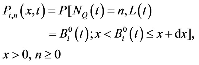
for and

We know that and, for . Also is continuous at. Then we have the hazard rate functions of as

(2.4)

where, and is the conditional probability of completion of i-th phase of service during the time interval, given that the elapsed service time is.

By assuming that the system is in the steady state, we let

(2.5)

for.

In the next section, we find the PGF of these probabilities.

3. The PGF of the System Size

Now, for, the PGF of the probabilities that explained by (2-5), are defined as

(3.1)

(3.2)

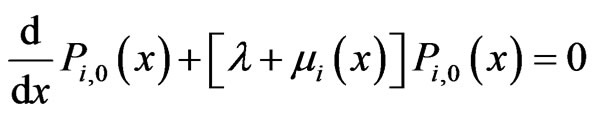
For finding the steady-state PGF from Kolmogorov forward equations, for, we can write the steady-state equations as

(3.3)

(3.4)

Also

(3.5)

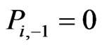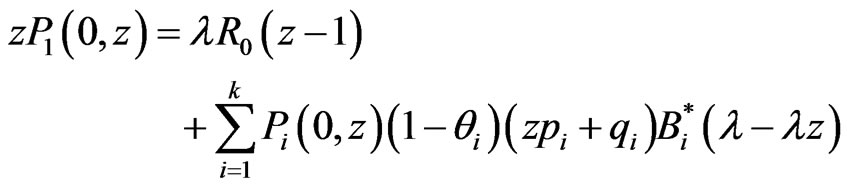
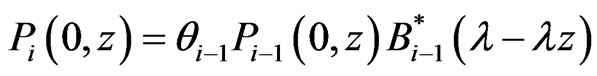
It is clear that, for. Now, at, the boundary conditions are

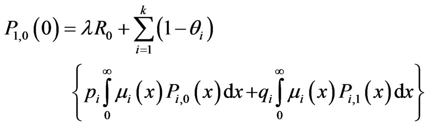(3.6)

(3.7)

(3.8)

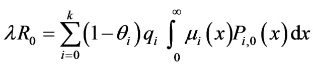
Note that, the normalizing condition is

which we use this condition to find the relation between and.

In the next Lemma, we derive the relation between and.

Lemma 3.1. From relation (3-3), we have 

(3.9)

Proof. See [4]. □

Proposition 3.2. By the z-transform of that is

we have

(3.10)

Proof. By multiplying the relation (3.7) in and summation from to, and using (3.6), the proof is completed.

Proposition 3.3. For, we have

(3.11)

Proof. By multiplying (3.8) in and summation on to , we can obtain (3.11).

Corollary 3.4. By proposition 3.3, we have

(3.12)

where

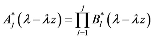(3.13)

Now, by (3.10) and (3.13), we obtain

(3.14)

Corollary 3.5. If, for , we have

(3.15)

and for

(3.16)

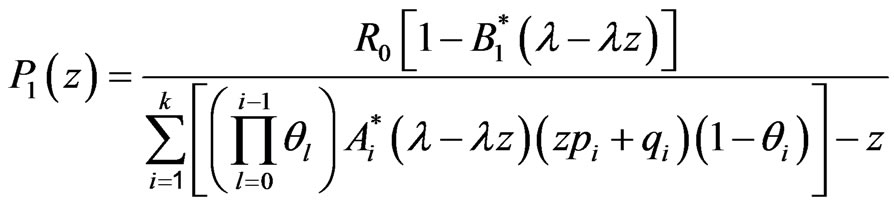
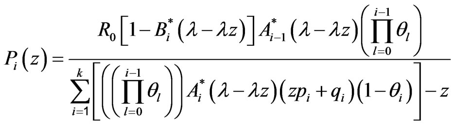
Now, if, and 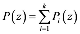is the PGF of queue size distribution at a random epoch, then from (3.15) and (3.16), we have

(3.17)

and the PGF of the queue size at the departure epoch is

(3.18)

In the next section, we find some measures of effectiveness as the means system size, response time and busy period. 

4. The Measures of Effectiveness

This section includes three sub-sections. In the sub-section 4.1, we find the mean system size. In the sub-section 4.2, the mean response time is obtained and in the last sub-section we calculate the mean busy period.

4.1. The Mean System Size

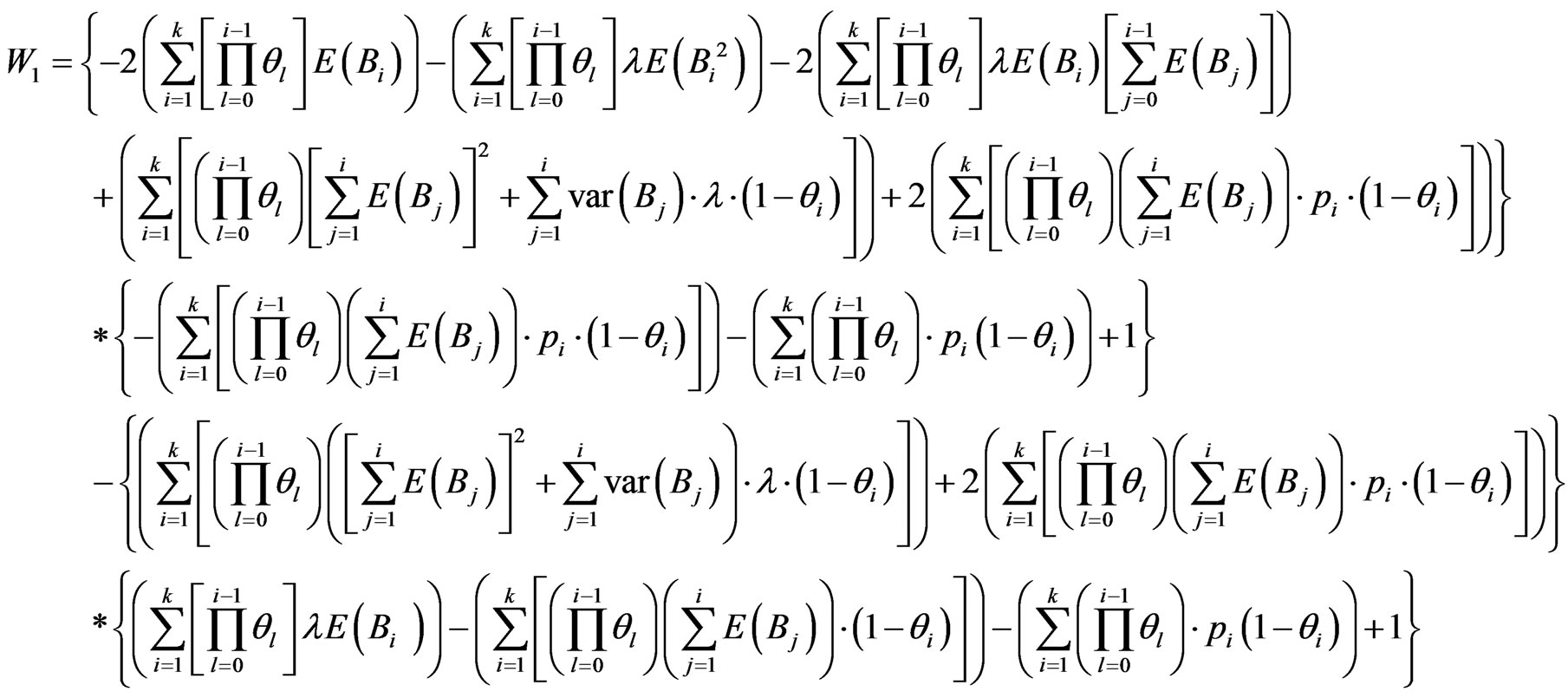
If be the mean number of customers in the queue, then we have

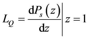
For calculating we use the following lemma.

Lemma 4.1.1. By (3.13) and for, we have 1)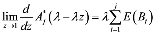(4.1.1)

2) 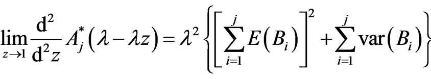(4.1.2)

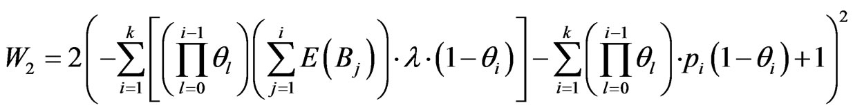
Now, we write in form ofwhere

and

Since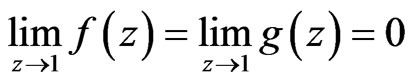, then by using the L’Hopital rule , we have

where

hence, in which

and

4.2. The Mean Response Time

Here, we show the response time variable with. For finding the mean of, first we need to obtain the LST of the distribution of waiting time in the queue, then by using this, we find the LST of the response time distribution. Then we can find the mean response time.

From classical formula in the queueing theory, we know that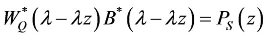, where

Now, if we put and using the (3.18), we have

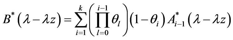
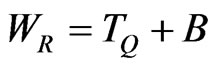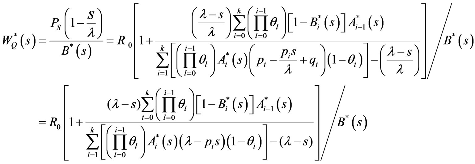
On the other hand, the response time is defined by, where is queueing time and is the service time. Then, by using the convolution property, the LST of is

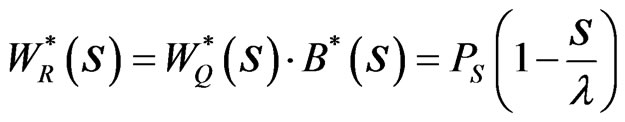
in which by some simple computation we find that

where

and

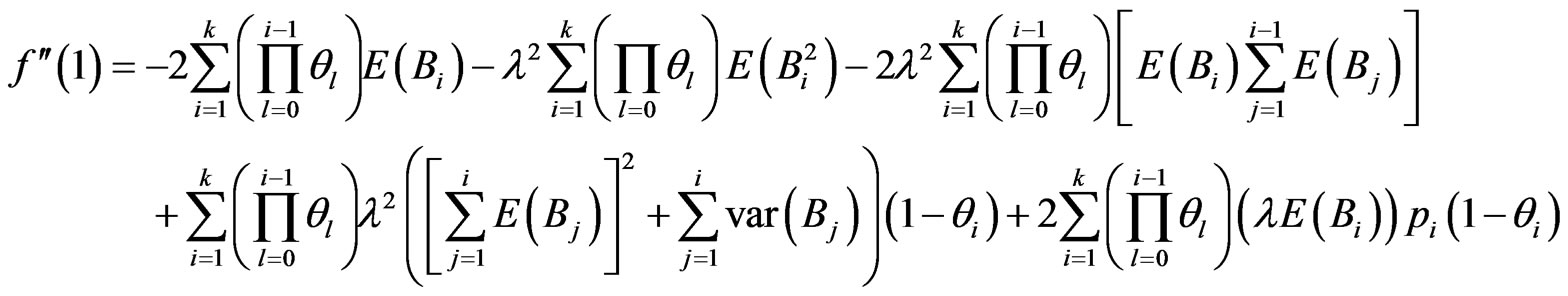
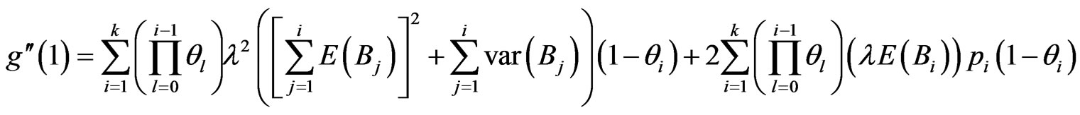
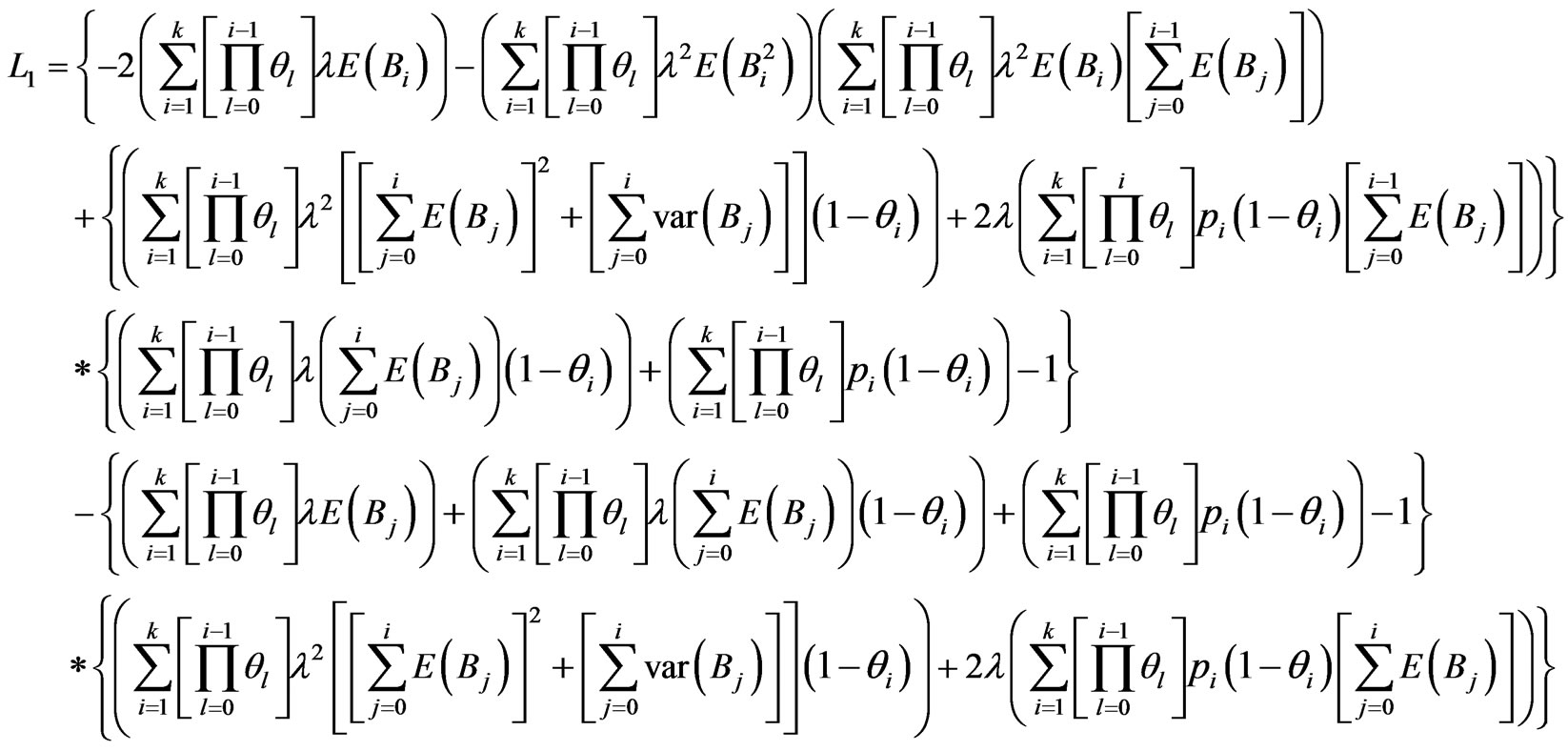
The mean response time, for an arbitrary customer, is

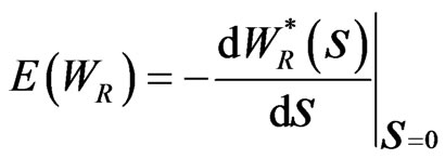
But, then, by using the L’Hopital rule, we have

(4.2.1)

On the other hand, and, then

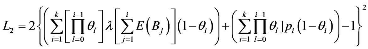
with replacing in (4.2.6), it results that

where 

and 

4.3. The Mean Busy Period

In this section, according to the definition of the busy period, we obtain the mean busy period of the model that we have studied here. Suppose that, and are the busy and idle periods, respectively. Now, according to the renewal theory, these variables are renewal processes and we have 

From this, it results

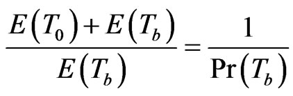
or

or

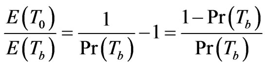
thus

Now, suppose that is the probability that the server is servicing in i-th phase that is P [the server is busy with (ps)_i], for

we have

Also, we know, then

4.4. Special Cases

In this article we have obtained some results for an M/G/1 queue with k-phases of heterogeneous services and Bernoulli feedback design. Now, we consider some special cases of this model that are agreement with the models which have been studied by [8,10]. These special cases are followed.

Special case 4.4.1. If, and the last phase be the vacation for server and without feedback, then, and are the same as those have been obtained by [10].

Special case 4.4.2. If and, then, , and are equal to the [4].

5. Conclusion

In this paper, we considered an M/G/1 queueing model with single server, Poisson input, k-phases of heterogeneous services and Bernoulli feedback design. In this model, as soon as the i-th (for i = 1, ∙∙∙, k − 1) phase of service of a customer is completed , it may leave the system or immediately go for (i + 1)-th phase of optional service. However, after receiving each phase of unsuccessful service by a unit, then it may immediately join to the end of tail of the original queue as feedback customer to take service again. We analyzed this mode via obtaining the steady-state probability generating function (PGF) of queue size at the random epoch and at the service completion epoch. Then, we derived the Laplace-Stieltjes Transform (LST) of the distribution of response time, the means of response time, number of customers in the system and busy period-model, the server provides first phase of regular service to all the customers.

REFERENCES

NOTES

¹First Come First Served.

REFERENCES

- D. Bertsimas and X. Papaconstantinou, “On the Steady State Solution of the M/C2(a;b)/s Queueing System,” Transportation Sciences, Vol. 22, No. 2, 1988, pp. 125- 138. doi:10.1287/trsc.22.2.125
- O. J. Boxma and U. Yechiali, “An M/g/1 Queue with Multiple Type of Feedback and Gated Vacations,” Journal of Applied Probability, Vol. 34, No. 3, 1997, pp. 773- 784. doi:10.2307/3215102
- G. Choudhury, “A Batch Arrival Queueing System with an Additional Service Channel,” International Journal of Information and Management Sciences, Vol. 14, No. 2, 2003, pp. 17-30.
- G. Choudhury and P. Madhuchanda, “A Two Phase Queueing System with Bernolli Feedback,” Information and Management Sciences, Vol. 16, No. 1, 2005, pp. 35-52.
- B. D. Choi, B. Kim and S. H. Choi, “An M/g/1 Queue with Multiple Types of Feedback, Gated Vacations and FCFS Policy,” Computers and Operations Research, Vol. 30, No. 9, 2003, pp. 1289-1309. doi:10.1016/S0305-0548(02)00071-0
- R. L. Disney, “A Note on sojourn Times in M/g/1 Queue with Instantaneous Bernoulli Feed-Back,” Naval Research Logistics Quarterly, Vol. 28, No. 4, 1981, pp. 679-684. doi:10.1002/nav.3800280415
- B. Krishna Kumar, A. Vijaykumar and D. Arivudainambi, “An M/g/1 Retrial Queueing System with Two Phase Service and Preemptive Resume,” Annals of Operations Research, Vol. 113, No. 1-4, 2002, pp. 61-79. doi:10.1023/A:1020901710087
- K. C. Madan, “An M/g/1 Queue with Second Optional Service,” Queueing Systems, Vol. 34, No. 1-4, 2000, pp. 37-46. doi:10.1023/A:1019144716929
- J. Medhi, “A Single Server Poisson Input Queue with a Second Optional Channel,” Queueing Systems, Vol. 42, No. 3, 2002, pp. 239-242. doi:10.1023/A:1020519830116
- G. H. Shahkar and A. Badamchizadeh, “A Single Server Queue with k-Phase of Heterogeneous Service under Bernoulli Schedule and a General Vacation Time,” Journal of Theoretical Statistic, Vol. 20, No. 2, 2006, pp. 151-162.
- H. Takagi, “A Note on the Response Time in M/g/1 Queue with Service in Random Order and Bernoulli Feedback,” Journal of Operational Research Society of Japan, Vol. 39, No. 4, 1996, pp. 486-500.
NOTES
1First Come First Served.