Journal of Biomedical Science and Engineering
Vol.7 No.9(2014), Article
ID:47938,16
pages
DOI:10.4236/jbise.2014.79068
An Efficient Numerical Method and Parametric Study for Electrolyte Transport in the Renal Medulla
Maryam Saadatmand1,2, Mohammad J. Abdekhodaie1*, Mahmoud R. Pishvaie1, Fathollah Farhadi1
1Department of Chemical and Petroleum Engineering, Sharif University of Technology, Tehran, Iran
2Department of Bioengineering and Robotics, Tohoku University, Sendai, Japan
Email: *abdmj@sharif.edu
Copyright © 2014 by authors and Scientific Research Publishing Inc.
This work is licensed under the Creative Commons Attribution International License (CC BY).
http://creativecommons.org/licenses/by/4.0/


Received 15 May 2014; revised 27 June 2014; accepted 10 July 2014
ABSTRACT
Mathematical models of the mamalian urine concentrating mechanism consist of a large system of coupled, nonlinear and stiff equations. An efficient numerical orthogonal collocation method was employed to solve the steady-state formulation of urine concentrating mechanism. This method was used to solve the stiff and high order equations of electrolyte transport in a central core, single nephron model of the renal outer medulla. The presented results were in good agreement with implicit finite difference method’s results, but this new method was faster and more stable. Due to the greater stability and larger convergence domain of collocation method over Newton’s method, a parametric study on concentrated urine was investigated. The results showed that this model was sensitive to non-ideal countercurrent exchange between medulla interstitium and vasa recta. Although distal tubule lies in the cortex interstitium, it affects on the inflow to the collecting duct. This study showed that the effect of changing membrane transport properties of distal tubule wall on properties of outflow from the outer medulla collecting duct was considerable.
Keywords:Urine Concentrating Mechanism, Central Core Model, Electrolyte Transport, Orthogonal Collocation, Parametric Study

1. Introduction
Mathematical modeling of the mamalian urine concentrating mechanism has been a matter of interest for many years [1] -[8] . These models have usually been formulated as steady-state boundary value problems (BVP’s) involving ordinary differential equations (ODE’s) expressing solute and water conservation in one space dimension corresponding to the cortico-medullary axis [1] . Since the nephron has a number of distinct tubules with different membrane transport properties, the equation set of urine concentrating mechanism for several constituents is a high order system [9] . Therefore, the steady-state model consists of a high order system of coupled and nonlinear ODEs [10] . Because of high values of hydraulic and solute permeability of some of the renal tubules, these equations are stiff. Introducing hydraulic pressure, electrical potential, and considering more solutes cause additional complications [2] [11] [12] . Hence, most models of renal concentrating mechanism have been formulated for NaCl and urea and treating NaCl as a nonelectrolyte solute instead of ionic species  and
and  [1] .
[1] .
In the most numerical methods, Newton-based methods [2] [13] [14] and quasilinearization in conjunction with a Newton-type solver [4] [15] have been used to solve the steady-state model of urine concentrating mechanism. However, these methods have difficulties with numerical instability which arises from reversal intratubular flow relative to the assumed steady-state direction [16] . This reversal of flow direction arises when transtubular water fluxes are large [5] . In addition, the convergence domain of Newton’s method is narrow and this method may converge if the initial estimate is sufficiently close to the steady-state solution [13] .
Dynamic formulation is an alternative approach to obtaining a steady-state solution. This formulation forms a system of coupled, nonlinear, hyperbolic partial differential equations (PDEs) and ODEs. Explicit methods such as upwind differencing or the ENO (essentially nonoscillatory) have been used to obtain the steady-state solution [17] . Although these methods eliminate numerical instability but due to the stiffness of the problem, they require small time steps causing a high computation cost [16] . Recently, the semi-lagrangian-semi-implicit method has been developed to obtain the steady-state solution to dynamic models of urine concentrating mechanism [16] [18] [19] . According to the lagrangian nature, it removes the numerical instability and due to the implicit nature large time scales can be used. Disadvantage of this method is complication of the programing and difficulty to modify model configuration for a large number of interacting tubules [16] .
The purpose of this work is to explain an efficient and stable method, based on orthogonal collocation scheme, to solve numerically the differential-algebraic equations (DAEs) arising in steady-state models of renal concentrating mechanism. Because of simplicity, inherent efficiency for applications to boundary value problems and optimal order accuracy for the error, the orthogonal collocation method is widely used [20] . In Newton-based methods, to minimize the truncation error which is introduced by converting differential equations to algebraic ones, the discretization number must be large. Therefore, these discretized equations form a large system of nonlinear algebraic equations. But in collocation method, the discretization points are selected such that the position of that points are optimal and thus the discretization number is not large. Consequently, collocation method is much faster than Newton-based methods. In addition, the convergency domain of orthogonal collocation method is not so small.
In this study, a model of electrolyte transport in outer medulla of mamalian renal system is presented using the orthogonal collocation method and the impact of important parameters on model results has been investigated.
2. Methods
2.1. Model
Most mammalian kidneys have three main sections: the cortex (C), the outer medulla (OM) and the inner medulla (IM) [21] . Within the cortex, the outermost layer of the kidney, fluid is essentially isosmotic to arterial blood. Whereas within the medulla, a cortico-papillary gradient of osmolality suffices to concentrate the urine [1] . The main functional units of the kidney are the tubular structures (with a radius on the order of 10 mm) called nephrons in which the urine is concentrated [22] .
In this work, the central core (CC) formulation proposed by Stephenson for electrolyte transport in a singlenephron of the renal outer medulla has been used [2] . This model includes a short-looped nephron with a loop of Henle (descending Henle’s loop (DHL) and ascending Henle’s loop (AHL)), a distal tubule (DT) and a collecting duct (CD). The central core model configuration is shown in Figure 1.
The loop of Henle and the CD may exchange with each other through the medulla interstitium (MI). In the central core model, all structures in medulla interstitium (e.g. interstitial cells, interstitial spaces and vasculature)
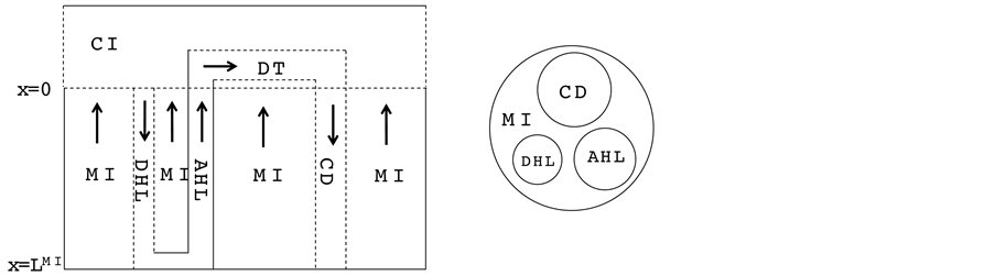
Figure 1. Schematic of central core model. Left: Tubules (DHL, AHL, DT and CD) and surrounding interstitium (CI and MI); Dashed lines: water permeable boundaries; Arrows: steady-state flow directions. Right: Medulla cross-section showing connectivity between MI and other tubules.
except Henle’s loop and CD are represented by a tubular compartment. The DHL, AHL, CD, and MI (superscripted by 1, 2, 4 and MI, respectively) are represented by rigid tubules that are oriented along the corticomedullary axis, which extends from x = 0 at the corticomedullary boundary to , at the boundary of inner and outer medulla. The DT (indexed by 3) that connect AHL to CD is shown by a rigid tubule located in the cortical interstitium (CI) [17] . Since
 ,
,  ,
,  and urea (subscripted by k = 1, 2, 3 and 4 respectively) are the most important solutes of renal medulla, these solutes have been considered in the presented model. The model formulations based on conservation of solute and water in renal outer medulla, predicts steady-state fluid flow rate, solute concentrations, electric potential and pressure profile as a function of the tubules and the OM lengths [2] .
2.1.1. Model Equations
In the steady-state, the water (approximately equal to solution flow) conservation equation for the i-th tubule of the nephron (I = 1, 2, 3, 4) is:
 (1)
(1)
where  is axial distance along the tubule,
  is axial water flow rate and
 ![]() is net outward transtubular water flux per unit tubular length.
is net outward transtubular water flux per unit tubular length.
It is assumed that the solutes are not being produced or consumed by chemical or physical reactions in any tubule, hence k-th solute (k = 1, 2, 3, 4) conservation for the i-th tubule (I = 1, 2, 3, 4) in the steady-state is represented by:
 (2)
(2)
where  is axial solute flow rate and
  is net outward transtubular solute flux per unit tubular length.
It is assumed that the pressure drop in each tubule can be explained by Poiseuille equation, therefore the pressure drop along the tubule i (I = 1, 2, 3, 4, MI) is determined by:
 (3)
(3)
where  is hydrostatic pressure and
  is flow resistance, in which
 ![]() is fluid viscosity and
is fluid viscosity and 
is tubule radius.
The transtubular fluxes are described by single barrier model equations which include a combination of different forces that exist between the tubule and the interstitium surrounding tubule (cortical interstitium for DT and medullary interstitium for DHL, AHL and CD). In general, both pressure gradient and osmotically driven forces determine the transtubular water flux across the tubular wall. Transtubular solute flux is determined by a combination of passive and active transport. Passive transtubular transport is described by Kedem and Katchalsky model [23] and simplified Goldman relationship for ionic fluxes [24] , while active transtubular transport obeys Michaelis-Menten kinetics. Therefore transtubular water flux, ![]() , and solute flux,
, and solute flux,  , can be written as:
 (4)
(4)
 (5)
(5)
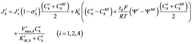 (6)
(6)
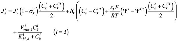 (7)
(7)
where for i-th tubule,  is hydraulic permeability,
 ![]() is passive permeability for k-th solute,
is passive permeability for k-th solute,  is Staverman reflection coefficient of the wall for the k-th solute,
  is concentration of k-th solute,
  is pressure and
  is electric potential relative to the cortical interstitium taken as the reference voltage and assumed to be zero. The last term in Equations (6) and (7) arises from active transport for k-th solute in i-th tubule,
is maximum rate of transport with  as Michaelis constant. In the above equations,
  is the universal gas constant,
  is the absolute temperature,
  is the Faraday constant and
 ![]() is the valence of the k-th solute.
is the valence of the k-th solute.
The water flux and solute flux equations for MI, arise from the transtubular water flux and solute flux from other tubules in medulla, are given by:
 (8)
(8)
 (9)
(9)
where i is summed over all tubules present in the medulla interstitium (I = 1, 2, 4). By integrating the combination of Equations (1) and (2) with Equations (8) and (9), two integrated mass balance for water flow rate and solute flow rate in the medulla have been obtained which mean that the sum of medullary water flow rate and solute flow rate at any depth are equal to the final collecting duct (CD) water flow rate and solute flow rate, respectively. Therefore, by using these integrated equations, water flow rate and solute flow rate at any level of medullary interstitium could be computed as:
 (10)
(10)
 (11)
(11)
where i is summed over all tubules exist in the medullary interstitium (i = 1, 2, 4),  and
and 
are the water flow rate and solute flow rate, respectively exiting from the CD.
In each tubule and medulla (I = 1, 2, 3, 4, MI), solute flow rate  is related to water flow rate
 concentration
  and potential
  by the Nernst-Planck equation:
 (12)
(12)
where  is the cross sectional area of the i-th tubule,
  is the diffusion coefficient of the k-th solute and
 ![]() is its mobility which is related to
is its mobility which is related to  by:
by:
 (13)
(13)
It has been assumed that in all tubules except the medullary interstitium, the diffusive term is negligible compared to the convective flow term. Therefore, the Nernst-Planck equation for tubules (i = 1, 2, 3, 4) simplifies to:
 (14)
(14)
Since ,
,  and
and  are ions, electroneutrality must be maintained according to the following equations (i = 1, 2, 3, 4, MI):
 (15)
(15)
 (16)
(16)
The cortical interstitium has been assumed to be a well-mixed bath of constant volume. Hence, solute concentrations, pressure and potential have been assumed constant in all cortical interstitium.
Therefore, the governing equations for the steady-state electrolyte transport model of a single nephron of the outer medulla consists of a coupled set of 35 differential equations (Equations (1)-(3)) and algebraic equations (Equations (10), (11), (15), (16)).
Since it is more convenient to work with dimensionless equations, dimensionless variables have been obtained by dividing dimensional variables by dimensional reference values. Specifically, dimensional  has been normalized through division by
 , that is i-th tubule’s length;
  by
by , which is the sodium concentration in fluid entering the DHL;
  by
by , that is water flow rate at the entrance of the DHL;
by , which is exit flow pressure from CD,
  by
by ; water flux
 ![]() by
by  which is the uniform rate of transtubular water transport for all of the water flow rate
  to exit through the walls of the i-th tubule; likewise,
  by
by , which means that all of solute flow rate,
  , exits through the i-th tubule’s wall at constant rate. The normalized parameters have also been obtained. Hence,
has been normalized through division by ;
; ![]() by
by ;
;  by
by ;
;  by
by 
and finally,  by
by .
.
2.1.2. Boundary Conditions
At the entrance of DHL, flow rate and solute concentrations have been given as the boundary conditions. The pressure at the entrance of DHL must be adjusted until the exit pressure for the CD has been defined. Likewise, solute concentrations, pressure and potential have been given for medullary interstitium at the cortico-medullary boundary. Stephenson et al. [3] showed that the effect of volume and solute flow rate to the outer medulla from the inner medulla, on the profiles of the outer medulla was negligible. As a consequence, this model was assumed to be closed at , i.e. there was no convective flow at
  in the medullary interstitium;
 . At the junction of nephron tubules, flow, solute concentrations and pressure must be continuous.
Because diffusion term was neglected in tubules, potential may be discontinuous at the junction of nephron tubules. The boundary conditions are given in Table1 The cortical interstitium constants and physical constants are given in Table2 Dimensional parameters, along with their units are listed in Table 3 [2] .
2.2. Numerical Procedures
The differential equations that describe flow and solute conservation and Poiseuille equation in central core model  can be represented in the general form of:
 (17)
(17)
The general form of algebraic equations for the flow and solute conservation of medulla and electroneutrality of central core model  are:
are:
 (18)
(18)
where  are the water and solute flow in tubules and pressure in tubules and MI and
  are water and solute flow in MI,
  concentration and electric potential in tubules and MI.
The collocation method is categorized in the weighted residuals methods to solve boundary value problems.
In which, the user provides an approximate solution and by substituting this solution into the governing equations, residuals will be calculated. Then one tries to force the residuals to be asymptotically close to zero. For the simple governing equations, user may provide an approximate solution that automatically satisfy the boundary conditions. For large and complicated governing equations, the residuals obtained by substituting the approximate solution in boundary equations should also be forced to be close to zero [25] . In this study, the Lagrangian interpolation polynomial has been used as an approximate solution to transfer the governing equations and boundary conditions to nonlinear algebraic equations at interior points and boundary points, respectively. Hence, the value of f (or g) at any point including the interpolation points, say![]() , is given by
, is given by
 (19)
(19)
 (20)
(20)
where  is the Lagrange interpolation polynomial and P is the number of interior (discretization) points. It should be noted that the type and location of boundary conditions are important for both the notation and implementation of method. For instance, if the value (and not the gradient) of differential quantity is known in upstream (at x = 0), the type of boundary condition is Dirichlet and the last point (i.e. the point number P + 1) is not included in the set of collocation points.
Although, the order of accuracy for collocation methods are known to be suboptimal, choosing appropriate interior points is critical to obtain optimal order of accuracy [20] . To solve the equations, each tubule and medulla were divided with P interior points (called collocation points) that were chosen as roots of an orthogonal Jacobi polynomial of P-th degree. The Jacobi polynomials are important in providing the optimum positions of the collocation points. For the orthogonality condition of the Jacobi polynomials the domain must be defined in the range [0,1]. Since the model equations have been converted to the dimensionless equations, all domains have been defined in the range [0,1]. By substituting these polynomials (Equations (17) and (18)) in the model equations and boundary conditions, a set of nonlinear algebraic equations have been obtained which can be solved by using any of algebraic solvers. Because the Broyden method requires only one function evaluation per iteration, it has been chosen to solve this system [25] . All calculations were performed using Fortran programs in double precision.
3. Results and Discussion
The electrolyte transport model in renal medulla has successfully been run by orthogonal collocation method. Since the condition number (the ratio of maximum eigenvalue to the minimum eigenvalue) of the jacobian matrix of the linearized model equations has been very large, it is obvious that electrolyte transport model in renal medulla is a stiff and high order equation set. Therefore, the finite difference method is not stable to solve this model. In contrast to finite difference method, the collocation method is faster and much more stable. In addition, the coupling of water and solute equations at junctions of tubules which is important in the urine concentrating mechanism, is more exact in orthogonal collocation method.
3.1. Convergence
The convergence of the results has been checked by increasing the discretization number and comparing some important quantities in urine concentrating mechanism. The water and solute balance in medulla, which are key scientific issues in numerical studies of urine concentrating mechanism, are always satisfied in this model. The medulla interstitium osmolality profile is shown in Figure 2 for different discretization number. Obviously, the difference between results with 10, 15 and 20 spatial grids is less than 1%, so each tubule and medulla interstitium has been divided into 10 segments.
3.2. Base-Case Profiles
The model equations (section 2) have been solved by orthogonal collocation method, using the base-case parameters (Table 2 and Table 3) and boundary conditions (Table 1) to obtain steady-state solutions for electrolyte transport in the renal outer medulla. Normalized water flow along the short looped nephron is shown
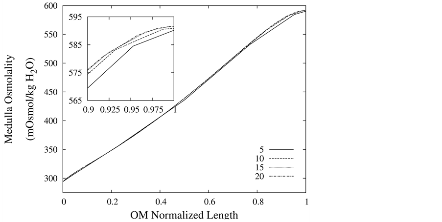
Figure 2. Medulla osmolality profile as a function of normalized medulla length, for different spatial grid size.
in Figure 3. Due to high hydraulic permeability of DHL and osmotic water absorption, outlet water flow rate from DHL decreases to approximately 50% of its input value. As a result of impermeability of AHL to water, AHL water flow rate is constant but negative, because fluid direction is toward the cortical interstitium, opposite to x direction. Due to osmotic water absorption, water flow rate reduces in DT and further in CD to a final normalized urine flow rate of 0.08. Similar to AHL, flow in MI is also negative.
Figure 4 and Figure 5 represent urea concentration and osmolality profiles along short-looped nephron. In these figures, profiles are in the same direction of flow in each tubule. Because of decreasing volume flow rate along the nephron, the urea concentration increases. Since urea is a waste product, the urea concentration in medulla interstitium is much lower than that in outflow from CD. MI osmolality at the boundary of inner and outer medulla is around twice plasma osmolality (591 mmol/kg∙H2O)) which is agree with the experimental data [2] . These results are consistent with Stephenson’s results [2] and physiological behavior of kidney. Therefore, assuming approximate solution of water and solute profiles in kidney as polynomials in orthogonal collocation method is consistent with the physiological behavior of the kidney.
3.3. Parametric Study
To perform parametric study for renal electrolyte transport model, a robust and stable solver is needed. Since the orthogonal collocation method is stable and has large convergence domain, the parametric study could be done perfectly using this method. The effect of membrane transport properties of distal tubule and non-ideality of medulla interstitium on properties of outflow from the outer medulla collecting duct (OM-CD) and medulla osmolality at the OM-IM boundary have been investigated. Since the distal tubule is in the cortex region of the kidney, it’s tubular fluid exchanges water and solute with cortical interstitium. Therefore, the influence of DT in central core model is only on the composition of inflow to CD at DT-CD junction. Most of the previous models did not simulate DT tubule and considered the fluid flow rate and composition entering to CD as boundary condition. Indeed, changing the inflow rate and composition to CD, changes outflow rate and osmolality.
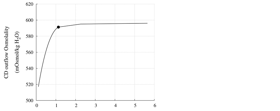
DT water permeability: Although, in the previous section the whole distal tubule has been considered water permeable, it has been confirmed experimentally that the early distal tubule is impermeable to water [26] . Thus, the effect of DT water permeability on CD outflow osmolality and MI osmolality at the OM-IM boundary have been studied (Figure 6). The presented results indicate that by increasing DT water permeability upto basevalue, CD outflow osmolality and medulla osmolality at OM-IM boundary increased. Increasing water absorption from DT resulted in increasing osmolality of inflow to CD. For base-case, as shown in Figure 5, osmolality
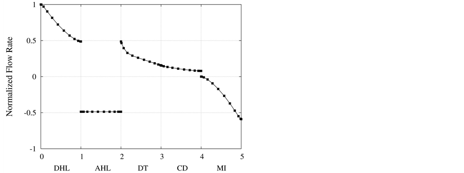
Figure 3. Normalized flow rate profile along short-looped nephron and outer medulla.
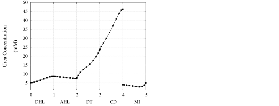
Figure 4. Urea concentration profile along short-looped nephron and outer medulla.
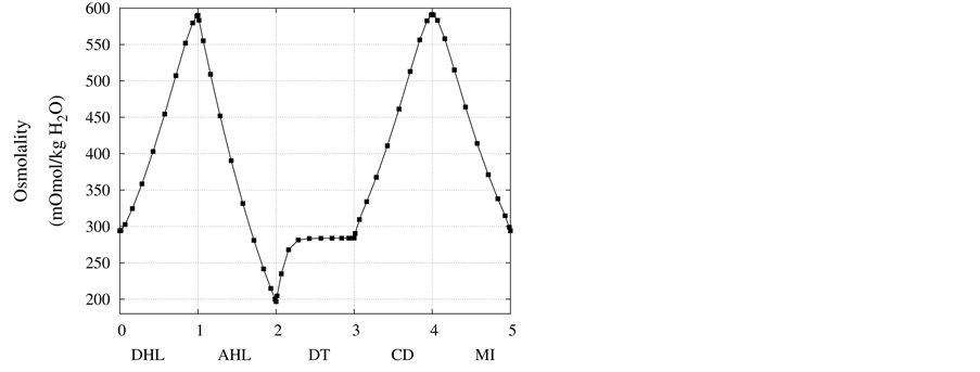
Figure 5. Osmolality profile along short-looped nephron and outer medulla.
at the end of DT was about , while cortex osmolality was constant at
 . As a resultsmall increases in DT water permeability from the base case value caused the osmolality in DT reached to the cortex osmolality. Experimental results also showed that the tubular fluid in DT approaches isotonicity to cortex fluid in the late portion of the distal tubule [27] .
DT active pump for  and
and : Most of NaCl exchanging between DT and cortical interstitium is performed by active transport [2] . Consequently, it is expected that the effect of switching off one or both of these active pumps, on simulated results is considerable. In Figure 7 and Figure 8, CD outflow osmolality and medulla osmolality at OM-IM boundary are shown for four different cases: 1) base-case, i.e. both active pumps are on with the parameters given in Table 3, 2) turning off
  active pump, 3) turning off
  active pump and 4) turning off both
  and
and  active pumps. By switching off active
  pump, the amount of
  in DT increased and thus lumen-positive potential increased and amount of
  decreased. Increasing DT
  concentration, resulted in increasing slightly fluid osmolality (not more than cortex osmolality) and reducing water absorbtion, thus caused increasing flow rate and osmolality of inflow to CD. As
  active pump was turned off, CD outflow osmolality and medulla osmolality at OM-IM boundary decreased. By switching off active
  transport, the amount of
  in DT increased and thus lumen became somewhat negative and amount of
  increased. Because of both pumps have the same strength (as given in Table 3), switching off
  or
or  has nearly the same effects on the presented results. In the other case, turning off both active pumps, caused increasing the amount of solute in DT and decreasing water absorbed from DT more than two last cases (turning off
  or
or  active pump). Indeed, active transport is an essential method to exchange solute between DT and cortex interstitium. Consequently, any problem in these pumps that causes to inactivate one or both of them, resulted in more water and solutes be excreted as CD outflow.
Nonideal countercurrent exchange in the medulla interstitium: In the blood supply of the kidney, there are a series of straight capillaries in the medulla named vasa recta. Each of the vasa recta lies parallel to the loop of Henle and has a hairpin turn in medulla. As noted previously, in central core model all vasculature and interstitium between tubules in medulla are represented by a tubular compartment. This representation assumes that countercurrent exchange between medulla interstitium and vasa recta is ideal. However, the transtubular permeabilities of the vasa recta to solute and water are not essentially infinite and countercurrent exchange between medulla interstitium and vasa recta is non-ideal and may hinder axial fluid and solute movement in MI. Often in central core models, nonideal vascular countercurrent exchange is represented by including axial diffusion term in solute flow equation (i.e. the diffusive term in the Nernst-Planck equation). These terms give a measure of the trapping of solute by the vascular counterflow system [2] . It is clear that in this term, diffusion coefficient of each solute is not equal to the diffusion coefficient of that solute in aqueous solution. The appropriate value of the diffusion coefficient for each solute depends on the flow rates and permeabilitis of vasa recta which are difficult to determine [3] . Diffusion coefficients used by Stephenson et al. [2] for solute diffusion in medulla interstitium are about an order of magnitude larger than corresponding values for solute diffusion in dilute aqueous solution [28] , whereas some researchers avoid this dissipative term [16] [18] . To illustrate the effects of nonideal countercurrent exchange in medulla interstitium, simulation with diffusion terms using diffusion coefficients that are factors of s = 0.1, 1, and 10 of the diffusion coefficients used by Stephenson [2] have been performed. Scaling factor 1 means that the diffusion coefficients are similar to those used by Stephenson et al. as base-case parameters (Table 3). Resulting values of important variables for CD outflow and medulla interstitium at the OM-IM boundary are given in Figure 9 and Table4 This table illustrates that the effect of the diffusion terms on results is considerable. As shown in Figure 9, osmolality profiles of MI is very sensitive to nonideal countercurrent exchange in medulla interstitium. By increasing nonideal countercurrent exchange, many of solutes in medulla are reabsorbed to blood flow in vasa recta, therefore medulla osmolality decreases. As a consequence of osmolality reduction of medulla, CD outflow osmolality decreases and CD outflow rate increases. These results illustrate that the effect of nonideal countercurrent exchange in medulla interstitium on OM-CD outflow concentrating is considerable. This means that any pathological problem that changes wall properties of kidney vasa recta will cause considerable changes in OM-CD outflow properties.
4. Conclusion
An efficient numerical solution based on orthogonal collocation method was presented to numerically solve the equations of electrolyte transport in a central core model of renal outer medulla. By considering three ions and urea as solutes and electrical potential in addition to other driving forces to exchange solute between tubule and
 (a)
(a)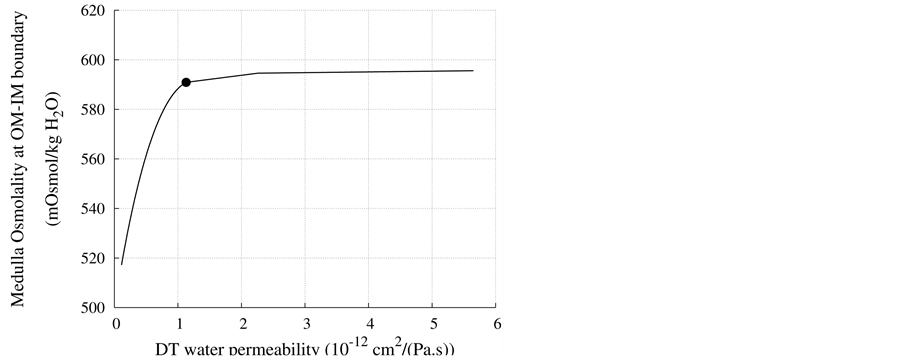 (b)
(b)
Figure 6. Effect of DT water permeability on CD outflow osmolality and MI osmolality at OM-IM boundary, : base-case value.
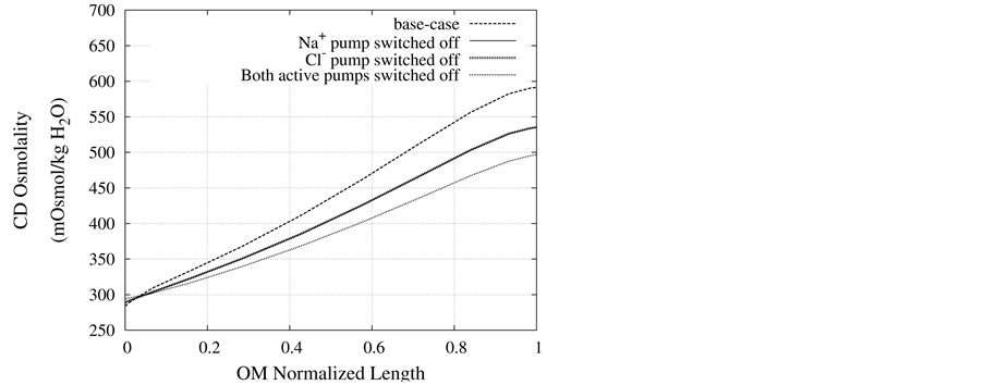
Figure 7. Osmolality profile along CD for different cases: a) base-case, b)  pump switched off, c)
  pump switched off, and d) both active pumps switched off.
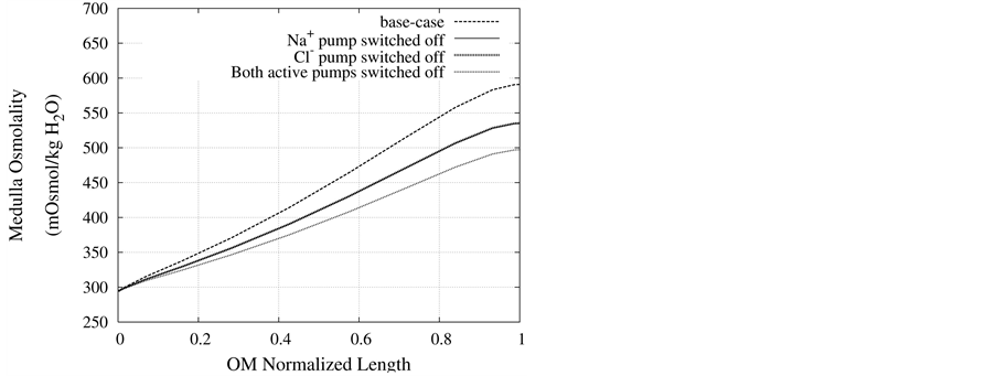
Figure 8. Osmolality profile along MI for different cases: a) base-case, b)  pump switched off, c)
  pump switched off, and d) both active pumps switched off.
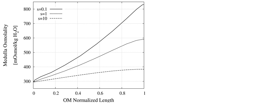
Figure 9. Effect of non-ideal countercurrent exchange in medulla interstitium on osmolality profile along MI.

Table 4. Effect of diffusion in medulla interstitium on normalized flow rate, solute concentrations and osmolality of CD outflow.
interstitium, this model contained a high order equation set. The orthogonal collocation method could successfully solve these complicated and stiff equations. Furthermore, orthogonal collocation method was faster and more stable than Newton’s method. Due to the greater stability and larger convergence domain of collocation method over Newton’s method, a parametric study on concentrated urine was investigated. The presented results indicated that the countercurrent exchange between medulla interstitium and vasa recta must be adjusted carefully in the central core model. Although distal tubule lies in the cortex interstitium, it affects on the inflow to the collecting duct. The presented results indicated that the effect of reduction of water permeability or any change in active pumps of DT wall on osmolality of CD outflow and also osmolality of medulla interstitium was considerable. It is believed that with help of this stable method, more complicated models such as inner medulla or 3-dimensional architecture of nephrons could be solved to obtain a better understanding of the mammalian urine concentrating mechanism.
References
- Layton, H.E. (2002) Mathematical Models of the Mammalian Urine Concentrating Mechanism, Membrane Transport and Renal Physiology. 129, Springer-Verlag, New York.
- Stephenson, J.L., Zhang, Y., Eftekhari, A. and Tewarson, R. (1987) Electrolyte Transport in a Central Core Model of the Renal Medulla. American Journal of Physiology—Renal Physiology, 253, F982-F997.
- Stephenson, J.L. (1972) Concentration of Urine in a Central Core Model of the Renal Counterflow System. Kidney International, 2, 85-94. http://dx.doi.org/10.1038/ki.1972.75
- Wexler, A.S., Kalaba, R.E. and Marsh, D.J. (1991) Three-Dimensional Anatomy and Renal Concetrating Mechanism. Modeling Results. American Journal of Physiology—Renal Physiology, 260, F368-F383.
- Thomas, S.R., Layton, A.T., Layton, H.E. and Moor, L.C. (2006) Kidney Modeling: Status and Perspectives. Proceedings of the IEEE, 94, 740-752. http://dx.doi.org/10.1109/JPROC.2006.871770
- Weinstein, A.M. (1994) Mathematical Models of Tubular Transport. Annual Review of Physiology, 56, 691-709. http://dx.doi.org/10.1146/annurev.ph.56.030194.003355
- Bykova, A.A. and Regirer, S.A. (2005) Mathematical Models in Urinary System Mechanics (Review). Fluid Dynamics, 40, 1-19. http://dx.doi.org/10.1007/s10697-005-0039-y
- Pannabecker, T.L., Dantzler, W.H., Layton, H.E. and Layton, A.T. (2008) Role of Three-Dimensional Architecture in the Urine Concentrating Mechanism of the Rat Renal Inner Medulla. American Journal of Physiology—Renal Physiology, 295, F1271-F1285. http://dx.doi.org/10.1152/ajprenal.90252.2008
- Wexler, A.S. and Marsh, D.J. (1991) Numerical Methods for Three-Dimensional Models of the Urine Concentrating Mechanism. Applied Mathematics and Computation, 45, 219-240. http://dx.doi.org/10.1016/0096-3003(91)90082-X
- Layton, A.T., Layton, H.E., Dantzler, W.H. and Pannabecker, T.L. (2009) The Mammalian Urine Concentrating Mechanism: Hypotheses and Uncertainties. Physiology, 24, 250-256. http://dx.doi.org/10.1152/physiol.00013.2009
- Stephenson, J.L., Zhang, Y. and Tewarson, R. (1989) Electrolyte, Urea, and Water Transport in a Two-Nephron Central Core Model of the Renal Medulla. American Journal of Physiology—Renal Physiology, 257, F399-F413.
- Stephenson, J.L., Zhang, Y. and Tewarson, R. (1976) Electrolyte, Urea, and Water Transport in a Two-Nephron Central Core Model of the Renal Medulla. Proceedings of the National Academy of Sciences, 73, 252-258. http://dx.doi.org/10.1073/pnas.73.1.252
- Mejia, R. and Stephenson, J.L. (1984) Solution of a Multinephron, Multisolute Model of the Mammalian Kidney by Newton and Continuation Methods. Mathematical Biosciences, 68, 279-298. http://dx.doi.org/10.1016/0025-5564(84)90036-1
- Tewarson, R.P., Stephenson, J.L., Garcia, M. and Zhanc, Y. (1985) On the Solution of Equation for Renal Counterflow Models. Computers in Biology and Medicine, 15, 287-295. http://dx.doi.org/10.1016/0010-4825(85)90012-5
- Wexler, A.S., Kalaba, R.E. and Marsh, D.J. (1991) Three-Dimensional Anatomy and Renal Concetrating Mechanism. Sensitivity Results. American Journal of Physiology—Renal Physiology, 260, F384-F394.
- Layton, A.T. and Layton, H.E. (2002) A Semi-Lagrangian Semi-Implicit Numerical Method for Models of the Urine Concentrating Mechanism. SIAM Journal on Scientific Computing, 23, 1526-1548. http://dx.doi.org/10.1137/S1064827500381781
- Layton, H.E., Pitman, E.B. and Knepper, A.M. (1995) A Dynamic Numerical Method for Models of the Urine Concentrating mechanism. SIAM Journal on Applied Mathematics, 55, 1390-1418. http://dx.doi.org/10.1137/S0036139993252864
- Layton, A.T. and Layton, H.E. (2003) An Efficient Numerical Method for Distributed-Loop Models of the Urine Concentrating Mechanism. Mathematical Biosciences, 181, 111-132. http://dx.doi.org/10.1016/S0025-5564(02)00176-1
- Layton, A.T., Pannabecker, T.L., Dantzler, W.H. and Layton, H.E. (2004) Two Modes for Concentrating Urine in Rat Inner Medulla. American Journal of Physiology—Renal Physiology, 287, F816-F839. http://dx.doi.org/10.1152/ajprenal.00398.2003
- Jator, S. and Sinkala, Z. (2007) A High Order B-Spline Collocation Method for Linear Boundary Value Problems. Applied Mathematics and Computation, 191, 100-116. http://dx.doi.org/10.1016/j.amc.2007.02.027
- Guyton, A.C. and Hall, J.E. (2006) Textbook of Medical Physiology. 11th Edition, Elsevier Saunders, Amsterdam.
- Sands, J.M. and Layton, H.E. (2009) The Physiology of Urinary Concentration: An Update. Seminars in Nephrology, 29, 178-195. http://dx.doi.org/10.1016/j.semnephrol.2009.03.008
- Kedem, O. and Katchalsky, Q. (1963) Permeability of Composite Membranes. Transactions of the Faraday Society, 59, 1931-1953. http://dx.doi.org/10.1039/tf9635901931
- Weinstein, A.M. (2002) A Mathematical Model of Rat Collecting duct 1.Flow Effects on Transport and Urinary Acidification. American Journal of Physiology—Renal Physiology, 283, F1237-F1251.
- Rice, R.G. and Do, D.D. (1995) Applied Mathematics and Modeling for Chemical Engineers. John Wiley and Sons, Inc., Hoboken.
- Schafer, J.A. (2000) Interaction of Modeling and Experimental Approaches to Understanding Renal Salt and Water Balance. Annals of Biomedical Engineering, 28, 1002-1009. http://dx.doi.org/10.1114/1.1308497
- Schafer, J.A. (2004) Experimental Validation of the Countercurrent Model of Urinary Concentration. American Journal of Physiology—Renal Physiology, 287, F861-F863. http://dx.doi.org/10.1152/classicessays.00020.2004
- (2001) CRC Handbook of Chemistry and Physics. 82nd Edition, CRC, Cleveland.
Nomenclature
i: Tubule or medulla superscript k: Solute subscript x: Medulla depth or DT length, cm
 : Water flow rate,
 : Solute flow rate,
![]() : Transtubular water flux,
: Transtubular water flux, 
 : Transtubular solute flux,
 : Electric potential, mV
 : Pressure, mmHg
 : Solute concentration,
 : Flow resistance,
 : Hydraulic permeability,
![]() : Solute Permeability,
: Solute Permeability, 
 : Reflection coefficient
 : Maximum transport rate,
 : Michaelis constant,
 : Diffusion coefficient,
![]() : Mobility,
: Mobility, 
![]() : Valence
: Valence
![]() : Viscosity, Poises F: Faraday constant,
: Viscosity, Poises F: Faraday constant, 
R: Universal gas constant, 
T: Absolute temperature, K
 : Radius, cm
 : Length, cm
 : Cross sectional area, cm2
NOTES

*Corresponding author.