Journal of Biomedical Science and Engineering
Vol.6 No.10(2013), Article ID:38352,9 pages DOI:10.4236/jbise.2013.610121
Optimizing feature vectors and removal unnecessary channels in BCI speller application
![]()
1Department of Biophysics, Zanjan University of Medical Sciences, Zanjan, Iran
2College of Electrical Engineering, Zanjan University, Zanjan, Iran
Email: *b.perseh@zums.ac.ir, majid_kiamini@yahoo.com
Copyright © 2013 Bahram Perseh, Majid Kiamini. This is an open access article distributed under the Creative Commons Attribution License, which permits unrestricted use, distribution, and reproduction in any medium, provided the original work is properly cited.
Received 16 August 2013; revised 12 September 2013; accepted 21 September 2013
Keywords: Brain Computer Interface (BCI); Speller Application; Event Related Potential (ERP); ERP Components; Channel Selection; Feature Extraction
ABSTRACT
In this paper we will discuss novel algorithms to develop the brain-computer interface (BCI) system in speller application based on single-trial classification of electroencephalogram (EEG) signal. The idea is to employ proper methods for reducing the number of channels and optimizing feature vectors. Removal unnecessary channels and reducing feature dimension result in cost decrement, time saving and improve the BCI implementation eventually. Optimal channels will be gotten after two stages sifting. In the first stage, the channels reduced up to 30% based on channels of the important event related potential (ERP) components and in the next stage, optimal channels were extracted by backward forward selection (BFS) algorithm. Also we will show that suitable single-trial analysis requires applying proper feature vector that was constructed by recognizing important ERP components, so as to propose an algorithm to distinguish less important features in feature vectors. F-Score criteria used to recognize effective features which created more discrimination between different classes and feature vectors were reconstructed based on effective features. Our algorithm has tested on dataset II of BCI competition III. The results show that we achieve accuracy up to 31% in single-trial, which is better than the performance of winner who is in this competition (about 25.5%). Also we use simple classifier and few channels to compute output performances while more complicated classifier and all channels are used by them.
1. INTRODUCTION
EEG is the brain activity record used widely as an important diagnostic tool in neurological disorder.
BCI systems are based on the analysis of the ERPs such as the P300 oddball event response [1,2]. ERPs are electrical superposition activities for more than a million neurons which reflected the brain response to stimulus (may be auditory, visual etc.) and because of concealed in EEG signal, EEG noise power is much higher than ERP or its signal to noise ratio which is −5 to −10 dB [3]. This factor causes ERP extraction task challenging. To achieve this task, numerous BCI competitions (such as BCI competition I, II, III, IV) are held (see website address: http://www.bbci.de/competition).
Various available data sets enable probes to figure out a new process for ERP extraction.
BCI system critically depends on several factors. For example we can mention cost, accuracy, how fast it can be trained and so on. Various methods and techniques are presented to achieve above factors. Generally, these methods can be separated into two categories:
• Optimal channel selection
• Proper feature extraction In the first category, the most common way is to use all channels (64 channels in the standard 10 - 20 system) for signal classification [4]. The major drawback of using this method is time computing which will be increased. Also, BCI system accuracy may be decreased.
In this study we will focus on a hybrid method which extracted optimal channels after two stages. In the first stage, we investigate the choice channels which have important components. These components such as P100, N200, P300 and etc… arise in stimulus response. Timing of these responses is latency brain’s communication time or information processing. For example the N200 explains as a negative voltage deflection occurring around 200 ms after stimulus onset, whereas the P300 component describes a positive voltage deflection occurring approximately 300 ms after stimulus onset. We indicated that all channels are unable to elicit all these components, so we present a method to select channels provided strong components from others.
Then in the next stage, optimal channels were extracted with backward forward selection (BFS) algorithm.
In the second part (i.e., proper feature extraction), we analyzed EEG signals with discrete wavelet transform (DWT) and wavelet coefficients which covered frequency range of lower than 15 Hz used for making feature vectors. Also, we eliminate some least significant features by using F-Score criteria. This approach results in reducing in feature dimension size (removal redundancy). So, classification accuracy for some trials has been increased considerably.
The rest of the paper is organized as follows: we’ll give an introduction to speller paradigm and data collection in Section 2, preprocessing algorithm described in Section 3, channel selection algorithm explained in Section 4 in detail. The feature extraction based on the wavelet transform is described in Section 5, and classification algorithm is described in Section 6. Experimental results are described in Section 7. Finally conclusion forms the last section.
2. SPELLER PARADIGM AND DATA COLLECTION
Speller paradigm described by [5] presents a 6 × 6 matrix of characters as shown in Figure 1. Each row or column is flashed in a random sequence. Task subject is to focus attention on characters in a word prescribed by investigator (i.e., one character at a time). Two out of 12 intensifications of rows or columns contain desired letter (i.e., one particular row and one particular column). The major problem is to predict letter by one of six columns and rows selection.
We applied a proposed method on data set II from third edition in BCI competition [6]. These data have been recorded with two different subjects. Each subject consists of 64 channels. Band-pass signals is filtered from [0.1 - 60] Hz and digitized at 240 Hz and with 15
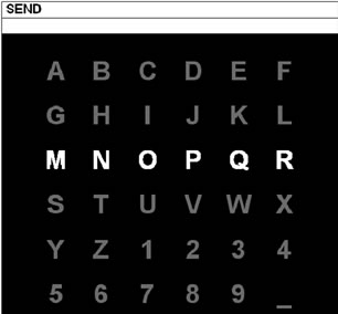
Figure 1. Speller paradigm screen.
repetitions per character. Each character is recognized with 12 stimuli, 6 columns and 6 rows [7].
Training and testing sets are made of 85 and 100 characters respectively. So, recorded signal numbers are: 85 × 12 × 15 = 15,300 and 100 × 12 × 15 = 18,000 for over all channels.
3. PREPROCESSING
In order to separate ERPs of target signals and non target signals, preprocessing operation will be done to identify more precisely components in EEG signal. Preprocessing, respectively, including:
• Filtering: signal has been filtered between [0.5 - 15] Hz by a 3− order Butterworth filter.
• Normalization: signal has been normalized by zero mean and unit variance.
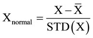 (1)
(1)
where X,  and STD(X) are EEG signal, which means value and standard deviation value of EEG signal respectively.
• Effective part of signal selection: samples in [0 - 700] ms posterior to intensification beginning (i.e., the first 168 samples) have been selected.
4. OPTIMAL CHANNEL SELECTION
In our speller application, spelling accuracy is function number of channels. In addition, with increasing number of channels cause great redundancy and accuracy reduction isn’t far from expected also. Therefore, channels must be chosen which limited. They are able to make strong ERP components, such as P100, N200 and P300 after a simple stimulus.
These optimal channels will be gotten after two sifting stages.
• Extraction of important channels for each component.
• Apply BFS algorithm.
4.1. Extraction of Important Channels for Each Component
Figure 2 shows typical grand average of target signal related to channels FC4, OZ and CZ for subject B. Grand average signal obtained from total target signals that averaged on train data. As you see P100, N200, and P300 components are clarity indicated in figure.
According to figure, it can be seen well around 100 ms channel FC4 and 300 ms channel CZ positive peak and around 200 ms channel OZ negative peak represented components P100, P300 and N200 respectively. Therefore, in central 100 ms, 200 ms and 300 ms with ±25 ms tolerance, it can be assigned intervals to recognize above components.

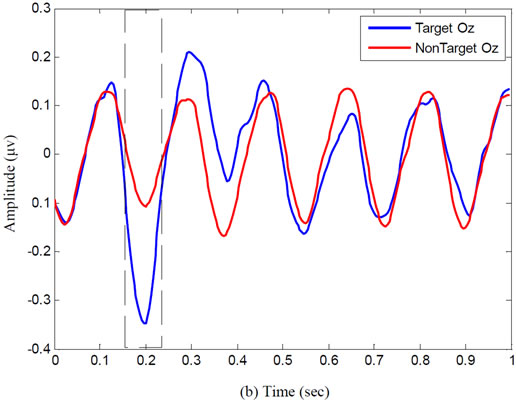
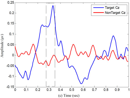
Figure 2. Typical ERP components waveforms: (a) P100 at electrode site; (b) N200 at electrode site; and (c) P300 at electrode site for subject B.
The purpose of this stage is to extract channels which are able to detect components very well. So, we take help from F-Score [8] distinction criteria. F-Score criteria are obtained in below:
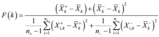 (2)
(2)
Typical ERP components waveforms: (a) P100 at electrode site, (b) N200 at electrode site, and (c) P300 at electrode site for subject B.
Where, 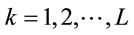 , L is the signal length,
  ,
,  and
and  are mean value of kth sample of target, non target and all respectively.
  is kth sample from ith target and
  is kth sample of ith non target.
  and
and  are number of target and non target signals respectively.
F-Score criteria calculate distinguishing between two data groups. If it gets higher, score will be larger than before. So, it is necessary to calculate F-Score value of each component from over all channels (for sample in time range defined as P100, N200 and P300). Then sum of scores value and the channel sort should be computed in decreasing order of scores. Important channels have been extracted by k channels which gotten highest scores. In Figure 3 for subject B, you can see F-Score value in all sample time related to channels FC4, OZ and CZ. According to this figure, there are peak scores around occurring important components.
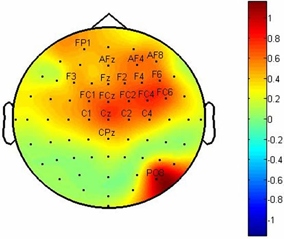
We marked twenty channels which have more abilities from others to identify components. Figures 4 and 5 show F-Score value topographies for subject A and B which calculated from P100, N200 and P300 components respectively. The output will be taken by gathering three channel sets which listed in Table 1. Note that some channels are repeated in channel sets.
According to Table 1, by applying F-Score criteria, we can reduce quantity of channels from 64 to 38 and from 64 to 44 for subject A and B respectively.
4.2. BFS Algorithm
This section purpose is to extract optimal channels from channels obtained in previous stage. The algorithm used is base on BFS. In each running stage of BFS algorithm, two channels are eliminated and one channel is added.
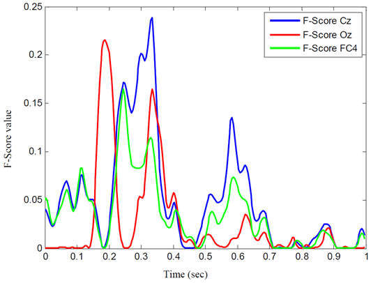
Figure 3. F-Score values of FC4, OZ, CZ and electrodes for subject B.
 (a)
(a)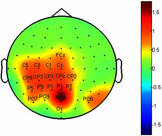 (b)
(b)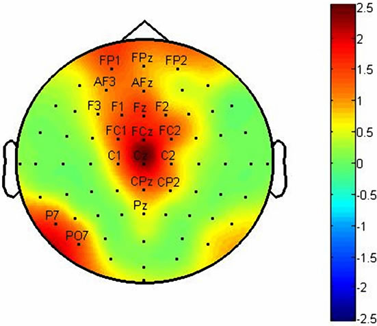 (c)
(c)
Figure 4. These figures show topographies values for F-Score in: (a) P100 latency; (b) N200 latency and (c) P300 latency for subject A.
 (a)
(a)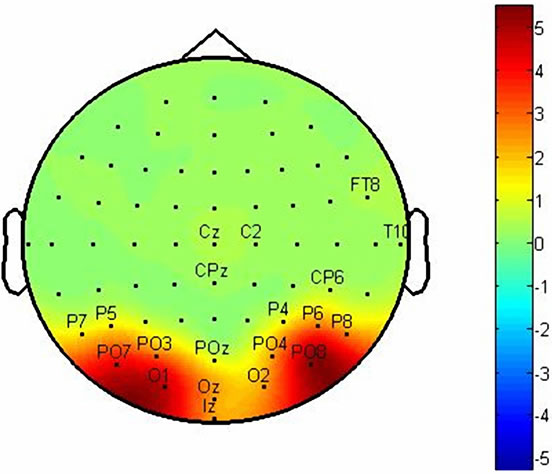 (b)
(b)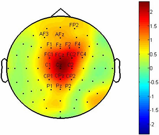 (c)
(c)
Figure 5. These figures show topographies of values of FScore in: (a) P100 latency; (b) N200 latency and (c) P300 latency for subject B.

Table 1. The list of channels which selected after two steps of channel selection. In first step, the channels selected base on ERP components and in second step, the optimal channels extracted with using BFS algorithm.
So, one channel will be reduced in each stage. Classification accuracy will be assessed on validation set described in the appendix.
BFS algorithm is implemented by following procedure:
1) Backward:
a) Calculate validation set accuracy by removing every one from each k channels on remains channels.
b) Find channel which has maximum bypass accuracy.
c) Eliminate implied channel. So, number of channels remain shall be equals to k − 1.
d) Run above process again. In this case, k − 2 channels are obtained.
2) Forward:
a) Add each eliminated channels separately to the obtained channel in backward section (include: k − 2 channels).
b) Find channel which maximized validation set accuracy by adding it. So channel quantity will be k − 1.
As you see, one channel in each stage of BFS must be reducing. This process will continue until number of channels equal to one. Now, we introduce channels are optimal channels which have higher validation set accuracy than others. This ranking procedure is sub-optimal, because always eliminated channels added just one channel, but not more.
Figure 6 shows results of BFS algorithm for subjects A and B.
As you can see, optimal channels are equal to 26 and 19 channels for subject A and B respectively which listed in Table 1.
Figure 7 shows electrode position of optimal channels for subjects under study.
5. FEATURE EXTRACTIONS
Feature extraction plays an important role for classification. Because of DWT ability to explore effectively of both time and frequency information [9,10], we apply wavelet usage to decompose EEG signal for calculating coefficients as define as feature vectors. The mother wavelet used was Daubechies order 4 which was deemed to be closest in to the signal waveforms. After decompo-
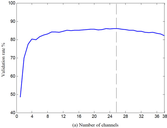
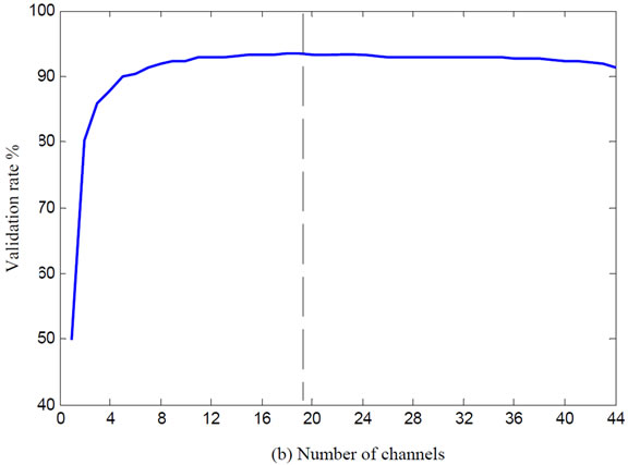
Figure 6. The variation of validation accuracy with respect to the number of channels. (a) Subject A and (b) Subject B.
sition up to five level, approximation coefficients of subband 5 and detail coefficients of subbands 5, 4 (i.e., [AC5 DC5 DC4]) are candidate for adding feature vectors.
According to Figure 2, creation structures and loss for major ERP components (such as P100, N200 and P300) aren’t same in different channels. Moreover in some channels these representatives are seen with larger peak or difference latency. In other words, we can say that after a simple stimulus, ERP signal is different from oth-
 (a)
(a) (b)
(b)
Figure 7. Topographical structures of channels selected for: (a) Subject A and (b) Subject B.
ers. So, we can conclude that above components don’t show themselves in same subband for different channels and all coefficients in subband don’t make enough discrimination between two classes also. Hence, using an algorithm for optimal coefficients choosing seems proper.
In this situation, redundancy reduced in feature dimension and discrimination between two classes can be increased also.
For meeting these requirements, we use a threshold level to discard less important features from feature vectors. Threshold level applies F-score value features which defined in (2). It allowed cutting features under threshold level. So, feature vectors will be reconstructed by remained features (i.e., features placed at above threshold level).
Threshold is defined for determining how amount feature percent must be eliminated. This limit is selected between intervals [10% - 60%] with 5% step increment. For choosing proper threshold, first we create feature vectors based on wavelet coefficients levels [AC5 DC5 DC4] for training set and calculate F-Score values in each attributes (i.e., wavelet coefficients). Then remove some value attributes which their scores are less than threshold level in [10%, 15%, 20%...60%]. After rebuild feature vectors based on remained coefficients for training set and validation set, we train classifier on training set and compute accuracy on validation set (more details are presented in appendix). So, threshold level will be defined as optimal threshold which maximizes validation set accuracy.
6. CLASSIFICATION ALGORITHMS
Fisher’s linear discriminant analysis (FLDA) classification is based on linear transform such that  (for classifying two or more classes [11]). Where W is discriminant vector, x is feature vector and y is output of FLDA. The major problem in FLDA is to compute the W vector. It may not be specified, when the features dimension becomes larger than the number of training data. Bayesian LDA (BLDA) is an expansion of LDA that can be seen as robust solution for this problem. In this study for regularization BLDA applied algorithm that presented in [12] which used the Bayesian least-squares support vector machine and Bayesian non-linear discriminated analysis. One can see in [12] more algorithm details. MATLAB implementation of BLDA is available in web page of EPFL BCI group (http://bci.ep.ch/p300).
7. EXPERIMENTAL RESULTS
In this section, simulated results are presented. It is necessary to compare results with others in competition. You can consider our proposed algorithms which evaluated on BCI competition III and data set II.
In channel selection section, optimal channels are extracted after two steps analysis. In first step, channels were labeled where they were gathered (Figures 4 and 5). We achieved 38 and 44 channels for subject A and B respectively. In other word, reduced channel rate is more than 30% after first stage. Channels are listed in Table 1. According to Table 1, a few channels as same between component channel sets (e. g, channel CZ are participated between P100 and P300 in two subjects) and more channels are different. The next step, optimal channels obtained as 26 channels for subject A and 19 channels for subject B under study. Figure 7 shows electrode position of them. Thereafter, we could reduce the feature dimension with a new initiation. So, feature vectors are reconstructed based on effective features with discarding less important features. To illustrate efficiency of proposed method in feature extraction, we evaluate two feature vectors as defined in Table 2. The results show that the proposed method reduces feature dimension while keeping higher accuracy in some trials. Classifier accuracy assessment is presented on Table 3 for both subjects with different trials.
Table 4 shows comparison between output accuracy
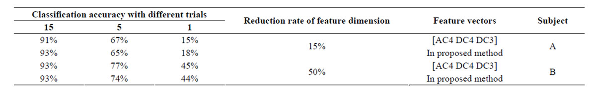
Table 2. Evaluation of two feature vectors (1—approximate coefficients level 5 and detail coefficients levels 5 and 4, 2—removal poor features and choose effective features) based on feature dimension and spelling accuracy.

Table 3. Classification accuracy for Subject A and Subject B with different trials.
of the best competitors in tournaments and results which have been obtained. Top results have been gotten from website: www.bbci.de/competition/iii/results. As you see, our results are better than second and third ranked competitors noticeably. According to reports by [13] (winners competition) in single trial, their precision is equal to 25.5%, but we achieved accuracy 31%. According to results, we can claim that proposed method improve performance in single trial in BCI speller application.
Another assessment is shown in Table 5. As you can see, using proposed method has advantages such as:
• Output accuracy meets only by average 22.5 channels, whereas number of channels is less than first.
• The paper results are obtained from simple classifier such as BLDA but first and second ones used support vector machine (SVM) classifier which is more complicated and processing time is higher than BLDA.
8. CONCLUSIONS
Three features can be defined as main key points for proper BCI system. These features are defined as low cost, real time response and high accuracy in BCI applications.
To achieve these key points, we propose methods for channel selection and feature extraction. We show that after a simple stimulus, more channels cannot create all important ERP components such as N200, P300 and P100 in EEG signal. But each component in some chan-
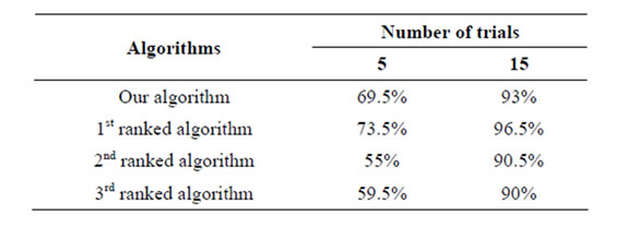
Table 4. Classification performance of our algorithm and three best competitors in BCI competition III (Data Set II).

Table 5. Evaluation of our proposed method. The best of three competitors’ algorithms in BCI competition based on number of channels and classification algorithm.
nels is seen independently. With this idea, we got optimal channels based on ones which created higher distinguishable channels in above components. We also use an algorithm to optimize feature vectors. Feature vectors (based on effective features) are created after eliminating the poor distinguishable features by F-Score criteria. Our experimental results show that proposed methods provided acceptable enhanced BCI system in speller application. After evaluation on data set II in BCI competition III, achieved accuracy is equal to 31% in a single trial and 93% in 15 trials. It seems that they are better than results reported by first and second ranked in this competition respectively.
REFERENCES
- Wolpaw, J.R., Birbaumer, N., Heetderks, W.J., McFarland, D.J., Peckham, P.H., Schalk, G., Donchin, E., Quatrano, L.A., Robinson, C.J. and Vaughan, T.M. (2000) Brain-computer interface technology: A review of the first international meeting. IEEE Transactions on Rehabilitation Engineering, 8, 164-173.
- Wolpaw, J.R. (2004) Brain-computer interfaces (BCIs) for communication and control: Current status. Proceedings of the 2nd International Brain-Computer Interface Workshop and Training Course, Graz, 17-18 September 2004, 29-32.
- Henning, G. and Husar, P. (1995) Statistical detection of visually evoked potentials. IEEE Engineering in Medicine and Biology, 14, 386-390.
- Liu, Y., Zhou, Z., Hu, D. and Dong, D. (2005) T-weighted approach for neural information processing in P300 based brain-computer interface. IEEE Conference on Neural Networks and Brain, Beijing, 13-15 October 2005, 1535-1539.
- Farwell, L.A. and Donchin, E. (1988) Talking off the top of your head: Toward a mental prosthesis utilizing eventrelated brain potentials. Electroencephalography and Clinical Neurophysiology, 70, 510-523. http://dx.doi.org/10.1016/0013-4694(88)90149-6
- Blankertz, B., Mller, K.R., Krusienski, D.J., Schalk, G., Wolpaw, J.R., Schlgl, A., Pfurtscheller, G., delRMilln, J., Schrder, M. and Birbaumer, N. (2006) The BCI competetion III: Validating alternative approaches to actual BCI problems. IEEE Transactions on Neural Systems and Rehabilitation Engineering, 14, 153-159. http://dx.doi.org/10.1109/TNSRE.2006.875642
- Schalk, G., McFarland, D.G., Hinterberger, T., Birbaumer, N. and Wolpaw, J. (2004) BCI2000: A general-purpose brain-computer interface (BCI) system. IEEE Transactions on Biomedical Engineering, 51, 10341043. http://dx.doi.org/10.1109/TBME.2004.827072
- Chen, Y.W. and Lin, C.J. (2003) Combining SVMs with various feature selection strategies. Studies in Fuzziness and Soft Computing, 207, 315-324. http://dx.doi.org/10.1007/978-3-540-35488-8_13
- Fatourechi, M., Birch, G.E. and Ward, R.K. (2007) Application of a hybrid wavelet feature selection method in the design of a self-paced brain interface system. Journal of Neuro Engineering and Rehabilitation, 4, 11. http://dx.doi.org/10.1186/1743-0003-4-11
- Yu, S.N. and Chen, Y.H. (2007) Electrocardiogram beat classication based on wavelet transformation and probabilistic neural net work. Pattern Recognition Letters, 28, pp. 1142-1150. http://dx.doi.org/10.1016/j.patrec.2007.01.017
- Fisher, R.A. (1936) The use of multiple measurements in taxonomic problems. Annals of Eugenics, 7, 179-188. http://dx.doi.org/10.1111/j.1469-1809.1936.tb02137.x
- Hofmann, H., Vesin, J.M., Ebrahimi, E. and Diserens, K. (2008) An efficient P300-based brain-computer interface for disabled subjects. Journal of Neuradcience Methods, 167, 115-125. http://dx.doi.org/10.1016/j.jneumeth.2007.03.005
- Rakotomamonjy, A. and Guigue, V. (2008) BCI competition III: Dataset II-ensemble of SVMs for BCI P300 speller. IEEE Transactions on Biomedical Engineering, 55, 1147-1154. http://dx.doi.org/10.1109/TBME.2008.915728
APPENDIX
We apply validation process base on five-fold crossvalidation method to obtain proper channels. The procedure is as follows:
1) Train data with 85 × 12 × 15 × ChannelCount signals (where, 85: characters, 12: stimuli, 15: time repetitions, and ChannelCount: number of channels) averaged over all signals by 3 time repetitions. So train data have been contained 85 × 12 × 5 × ChannelCount signals.
2) We divide 85 characters to five partitions and built validation set from N × 12 × 5 × ChannelCount signals, where, N contain 17 characters and use the residual data to form a training set.
3) Feature vectors created base on wavelet coefficients (approximate coefficients level 5 and detail coefficients levels 5 and 4 ([AC5 DC5 DC4]).
4) Training set train on BLDA classifier and output precision evaluate on validation set. The precision is defined as , where TP, FP, FN are the number of true positive, false positive and false negative, respectively.
5) Validation performance has been assessed by averaging between five precisions.
NOTES
*Corresponding author.