Journal of Geographic Information System
Vol.5 No.2(2013), Article ID:30251,17 pages DOI:10.4236/jgis.2013.52017
Application of LiDAR Data for Hydrologic Assessments of Low-Gradient Coastal Watershed Drainage Characteristics
1USDA Forest Service, Cordesville, USA
2Gainesville State College, Oakwood, USA
3University of Georgia, Athens, USA
Email: damatya@fs.fed.us
Copyright © 2013 Devendra Amatya et al. This is an open access article distributed under the Creative Commons Attribution License, which permits unrestricted use, distribution, and reproduction in any medium, provided the original work is properly cited.
Received January 25, 2013; revised February 26, 2013; accepted March 20, 2013
Keywords: Santee Experimental Forest; Digital Elevation Models (DEM); Drainage Area; Drainage Network; Low-Gradient Coastal Plain (LCP)
ABSTRACT
Documenting the recovery of hydrologic functions following perturbations of a landscape/watershed is important to address issues associated with land use change and ecosystem restoration. High resolution LiDAR data for the USDA Forest Service Santee Experimental Forest in coastal South Carolina, USA was used to delineate the remnant historical water management structures within the watersheds supporting bottomland hardwood forests that are typical of the region. Hydrologic functions were altered during the early 1700’s agricultural use period for rice cultivation, with changes to detention storage, impoundments, and runoff routing. Since late 1800’s, the land was left to revert to forests, without direct intervention. The resultant bottomlands, while typical in terms of vegetative structure and composition, still have altered hydrologic pathways and functions due to the historical land use. Furthermore, an accurate estimate of the watershed drainage area (DA) contributing to stream flow is critical for reliable estimates of peak flow rate, runoff depth and coefficient, as well as water and chemical balance. Peak flow rate, a parameter widely used in design of channels and cross drainage structures, is calculated as a function of the DA and other parameters. However, in contrast with the upland watersheds, currently available topographic maps and digital elevation models (DEMs) used to estimate the DA are not adequate for flat, low-gradient Coastal Plain (LCP) landscape. In this paper we explore a case study of a 3rd order watershed (equivalent to 14-digit hydrologic unit code (HUC)) at headwaters of east branch of Cooper River draining to Charleston Harbor, SC to assess the drainage area and corresponding mean annual runoff coefficient based on various DEMs including LiDAR data. These analyses demonstrate a need for application of LiDAR-based DEMs together with field verification to improve the basis for assessments of hydrology, watershed drainage characteristics, and modeling in the LCP.
1. Introduction
Watersheds are an organizing framework for the assessment of hydrologic and ecological functions and various impacts of the landscape. Reliable and sustainable water yield from watersheds in the Southeastern Coastal Plain has become an area of concern in recent years because of changing population growth, land use, and potential climate change. To address this concern, there is a need for a reliable understanding of hydrologic processes and water balance of less disturbed, forested watersheds on low-gradient Coastal Plain (LCP) lands [1-7]. This reference water balance could be used to quantify the magnitude and potential change to water balance in the LCP due to the impacts of human and natural disturbances, which is important for economic development and land management practices. Resource data (e.g., topography, hydrography, land use/land cover, soils) characterizing the watersheds are the basis for those assessments, and its resolution may affect results and interpretations. Monitoring and modeling approaches are often used to understand the processes and quantify the runoff, water balance, and pollutant loads [8]. However, there are challenges in accurately quantifying the water and chemical balance of these LCP systems primarily due to the difficulty in accurately estimating the watershed drainage area used in depth-based runoff.
The drainage area can be estimated with a reasonable accuracy for high-gradient upland watersheds with regularly available US Geological Survey (USGS) topographic quadrangle maps (Scale 1” = 1 mi with 20-ft contour intervals) or digital elevation models (DEMs). Most of the analyses in the study were conducted using USGS topographic-quad map based DEMs. The DEM is a digital cartographic/geographic dataset of elevations in xyz coordinates. The terrain elevations for ground positions are sampled at regularly spaced horizontal intervals. DEMs are derived from hypsographic data (contour lines) and/or photogrammetric methods using USGS 7.5-minute, 15-minute, 2-arc-second (30- by 60-minute), and 1-degree (1:250,000-scale) topographic quadrangle maps.” http://tahoe.usgs.gov/DEM.html. The 30 m DEM developed from hypsographic data (contour lines) and/or photogrammetric methods using the 7.5’ USGS topographic quadrangle map is generally the hydrologists’ choice for watershed drainage area delineation [9,10]. However, more accurate topographic maps may be needed to obtain an accurate estimate of the drainage area in the LCP where the land slope is very flat with a few contours. For example, recently [11] found huge discrepancies in the elevation data of Interstate (I-95) obtained by 10 m DEM created from 10 m contours developed by hand digitization of USGS 1:24,000 scale topographic maps compared to the DEM developed from the 2010 Light Detection and Ranging (LiDAR) data. The older 10 m DEM and the latest LiDAR-DEM provided an average difference of 0.9 m on randomly selected locations on the I-95. They converted the 10 m DEM for the study area (Camden County, GA, a southern coastal county) using the algorithm developed with differentiation values of both. The study area, USDA Forest Service Santee Experimental Forest (SEF), used in this study is of similar topographic nature. Similarly, [12] reported that the USGS topographic maps are considered insufficiently accurate in their topographical representation of watershed boundaries, slopes, and upslope contributing areas to meaningfully apply detailed processbased soil erosion assessment tools at the field scale. However, the authors also concluded that DEMs based on USGS 10-ft contour lines from publicly available data can be as good as the most accurate datasets obtained from real-time kinematic differential GPS (RTK-DGPS) in estimating average annual off-site runoff (−18.3% error) and sediment yield using the WEPP model within a 30- ha upland watershed. Most recently, [13] reported the effects of uncertainty in estimating elevations from various DEM types on erosion rates. Similarly, in another study by [14], the authors argued that it is often difficult to quantify soil loss due to gully erosion because the footprint of individual gullies is too small to be captured by most generally available DEMs, such as the USGS National Elevation Dataset. James et al. [15] also noted that the standard DEMs generally lack the spatial and temporal resolution to perform change detection at the local gully scale. Depending on data sources, methods and procedures used to generate field DEMs, the DEM estimates contain errors [16]. Thus LiDAR data are being increasingly used to derive information on elevation [17]. However, only a very few or no studies have been conducted so far on the effects of errors in DEMs in estimating drainage area of watersheds in low-gradient coastal landscapes (LCP).
DEMs created using elevations from the USGS topographic quad maps may often be altered by construction of roads and cross-drainage structures, more so in flat LCP. In these flat lands such a road bed may serve as a boundary of the watershed that may not have been reflected in the old USGS topographic map based DEMs [18]. If not field verified for those road infrastructures and reconditioned in the DEM, the actual estimated drainage area as well as drainage network may well be different from that developed using the available DEMs. This clearly suggests a necessity for field investigation of road network and other flow control structures in addition to having accurate high resolution DEM for hydrologic analysis and modeling, especially that involves drainage area calculation, in coastal plains.
In this paper we illustrate how the recognition of historical land use features, including water management structures, as a result of high resolution spatial data, affects our understanding of hydrologic processes and pathways. We provide examples of hydrologic models to illustrate how the resolution of the resource data (e.g., soils, vegetation, land use, topography, and hydrography) used as model inputs and the model design may affect interpretations. Most process based models require some form of calibration and/or validation prior to their applications [8,19-21]; that calibration process typically involves modifying parameters or coefficients for specific processes to achieve reasonable model performance with respect to the output of interest. The assumption is that reasonable agreement between the simulated and measured data (e.g., stream discharge) reflects an accurate representation of the processes within the watershed. However, seemingly accurate predictions of stream flow at the watershed outlet may be achieved by complementary errors from internal processes resulting in inaccurate predictions of in-stream flows, water table depths, and soil moisture within the watershed [19].
Floodplains in the Coastal Plain of the southeastern United States were the principal agricultural zone during the early colonial era (e.g., late 1600’s and early 1700’s). In South Carolina, the freshwater floodplains were used for rice cultivation. The development of the land included water management features like reservoirs, impoundments, diversion and distribution channels, diked fields, and lateral ditches and collector canals [22]. Those manmade features remain on the landscape, however they are not apparent in the classical resource data used for hydrologic assessments and modeling [9,23]. Thus the current USGS topographic survey information is of insufficient resolution to demark these important land features affecting hydrologic pathways and functions as well as to delineate the LCP watersheds.
The objectives of this paper were: 1) to analyze LiDAR data and summarize field observations of the stream channel network and other various drainage and legacy water management features on the Santee Experimental Forest, South Carolina and 2) to summarize the effects of various topographic maps and DEM resolutions used in estimating drainage area on average annual runoff coefficient for a forested watershed (Turkey Creek) in the Atlantic Coastal Plain. Furthermore, the effects of roads and road culverts on estimated actual effective drainage area using the available DEM are also discussed in the manuscript.
2. Materials and Methods
2.1. Site Description
2.1.1. Santee Experimental Forest
This work was conducted on the US Forest Service’s Santee Experimental Forest (SEF) in South Carolina. The SEF is representative of the lower Coastal Plain landscape (LCP), characterized by low relief, mixed hardwood-pine flatwoods, and bottomland hardwood floodplains. The SEF was part of the Cypress Baroney that was conveyed by King Charles in 1697; the land was subsequently divided into three plantations in 1707, which is when the agricultural development began. The floodplains of first, second and third order streams were developed into rice fields during the early 1700’s period. The present topographic, hydrography, soils and vegetative information for the forest convey a uniform, lowrelief landscape (Figure 1). These are the typical spatial data that are used for hydrologic modeling [1,8,21].
LiDAR data for the SEF were obtained using Airborne
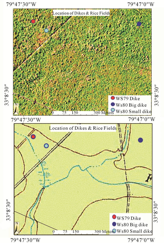
Figure 1. The aerial photograph, and USGS topographic map (1:24,000), of a section of the Huger Creek, Santee Experimental Forest.
Laser Terrain Mapping technique in 2007 by [24]. The raw LiDAR data were collected with a horizontal resolution of 0.1 m and a vertical accuracy of 0.07 - 0.15 m. The bare-earth return data were processed in ArcGIS to smooth the DEM and map potential stream channels using the ArcHydro extension (flow direction, length).
2.1.2. Turkey Creek Watershed
Most of the Turkey Creek watershed is in the Francis Marion National Forest on the coastal plain of South Carolina (Figure 2) with a small downstream portion including the gauging station within the Santee Experimental Forest. The US Forest Service established a stream gauging station in Turkey Creek in 1964 and monitored the watershed until 1984 only. Nevertheless, researchers recognized the importance of stream gauging and other hydro-meteorological data from a forested coastal watershed as a reference in a rapidly changing coastal environment. As a result, in 2004, the US Forest Service, in cooperation with the College of Charleston and the USGS, reinstalled a real-time streamflow and rain gauging station, (http://waterdata.usgs.gov/sc/nwis/uv?site_no=02172035) approximately 800 m upstream of the historic gauging station [25].
The study watershed is located within the USGS quadrangle maps of Huger (NE), Bethera (SE), Shulerville (SW and SE), and Ocean Bay (NW and NE) with the approximate coordinate ranges of 610,400 to 628,600 easting and 3,658,500 to 3,670,500 northing [1].
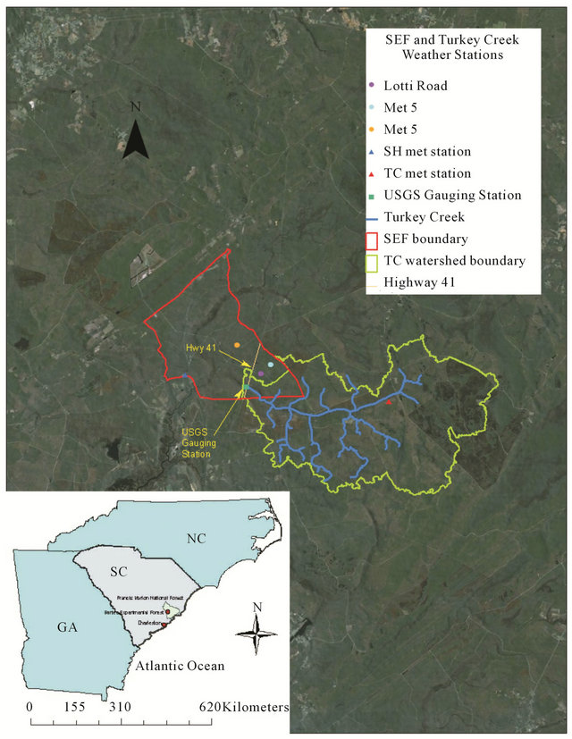
Figure 2. Location of the Turkey Creek watershed (green boundary) adjacent to the Santee Experimental Forest (red boundary) in coastal South Carolina (SC), also shown are the monitoring stations in and around the watershed.
Located within a 12-digit hydrologic unit code (HUC 030502010301) of the Catawba-Santee basin [26] at the headwaters of East Cooper River, a major tributary of the Cooper River draining to the Charleston harbor system, Turkey Creek (WS 78) is typical of other watersheds in the south Atlantic Coastal Plain, where rapid urban development is taking place. Technically, Turkey Creek is a 6th level hydrologic unit that qualifies only as a subwatershed although we refer to it as a “watershed” in this paper. The topographic elevation of the watershed varies from about 2.0 m at the stream gauging station to 14 m above mean sea level [1].
2.2. Evolution of Drainage Area
The estimation of drainage area of the Turkey Creek watershed changed as more accurate maps and associated DEMs were available in the course of this 48-year (1964-2011) period (Table 1). When the watershed was established in 1964, the drainage area boundary was approximated using the then available USGS topographic map with a scale of 1 inch = 2 miles. Later on in early 1969 the 1 inch = 1 mile scale USGS map was used to obtain a new boundary and watershed area. Although flow data on the watershed were continuously collected until 1984, no analysis or publication was done with these historic data, except for internal station reports. After discontinuation of flow measurements in 1984, it was not reestablished until late 2004. Accordingly, there were not any updates in drainage area of the watershed although new DEMs continued to become available in the late 80’s and 90’s.
The first literature search on recent DEMs in late 2004, when the Turkey Creek watershed was reestablished, resulted in a 1999 publication for 14-digit hydrologic unit code (HUC) development for South Carolina [26] which used the 1:24,000-scale 7.5-minute series topographic maps as the source maps and the base maps from 1:100,000-scale Digital Line Graphs; however, the data
Table 1. Drainage areas and calculated average annual runoff coefficients (ROC) for Turkey Creek watershed based on map or DEM types used during 1964-2011 period.
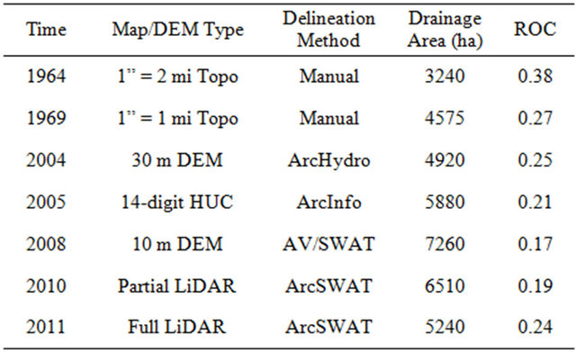
were published at a scale of 1:500,000. In the 2005 Hydrologic Unit Code (HUC) map for South Carolina [26], Turkey Creek area was listed as 6685 ha (16,508 ac) to its confluence with Nicholson Creek, which is further downstream from the current gauging station. The source maps for the basin delineations using the HUCs are 1:24,000-scale 7.5-minute series topographic maps, and 1:24,000-scale digital raster graphics. Same map was used by the USGS to delineate the area at the current gauging station on Highway 41N near Huger. Similarly, DEMs with 30 m horizontal resolution and 1 m vertical resolution were also available from SC Department of Natural Resources in 2004. Later in 2006, the USGS Enhanced 1:24,000 true 10 m horizontal 1 m vertical DEM was obtained from the USGS [28]. The crossdrainage structures on forest roads in and around the Turkey Creek watershed were also surveyed using 3-D Delorme topographic quad maps of 2002 [29] with a scale of 1:25,000 and a 1988 Forest Service Francis Marion National Forest map with a scale of 1:126,720 that showed perennial streams, bridges, and road names. The field equipment included a GPS unit-Garmin GPS V personal navigator (with an accuracy of 6 - 9 m), a digital camera, a 50 m measuring tape, and a compass during December 2006-April 2007 period. The details of the field survey results of cross-drainage structures (44 culverts) are given by [28].
The LiDAR data obtained in 2007 for Santee Experimental Forest [30] also contained a small part of the downstream portion of the Turkey Creek watershed adjacent to the Forest (Figure 2). This was available in very high resolution DEMs (at a 2 m point spacing or better, and gridded with a 1 m resolution and a vertical accuracy of 0.07 - 0.15 m). The estimate of drainage area was updated using DEMs covering that smaller area with LiDAR data. Finally, by August 2011, similar high resolution LiDAR data (draft only) for the Berkeley County, SC containing the whole Turkey Creek watershed was obtained from the SC Department of Natural Resources (SCDNR) [31].
The specifications of the LiDAR elevation data acquired as point cloud (“LAS”) for the Turkey Creek watershed included a nominal point spacing of 1.5 meter and vertical root mean square error (RMSE) of 18.4 cm (Figure 3). The vertical RMSE suggests that there is a possibility of 18.4 cm average error in elevation in the DEM created from the LiDAR data. Quick Terrain Modeler® ×64 [32] was used to generate the bare earth ground and water surface raster DEM with a cell size of 1.5 m. Although the LiDAR data resolution was 0.3 m, the DEM of 1.5 m resolution was developed to reduce the file size and thus promote faster analysis. The generated DEM was then exported as an ERDAS IMAGINE image [33] and projected to State Plane NAD-83-South Carolina
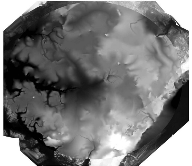
Figure 3. LiDAR-based DEM of 1.5 m × 1.5 m horizontal and 0.18 m vertical resolution.
FIPS 3900 feet, using ESRI® ArcGIS 9.3.1 [34].
2.3. LiDAR-DEM Reconditioning for Culverts
The DEM was further pre-processed to minimize generation of discontinuous streams due to presence of bridges and culverts. Additional challenges of working with low relief and very low slope watersheds such as Turkey Creek are such that wide areas can have a slope of near zero and the area is covered by a network of raised and compressed logging and forest service road beds. These effectively act as runoff barriers or miniature dams. To address some of these challenges, a comprehensive culvert survey of the study area was carried out in 2010 and 2011 using a combination of identifiers to predict the likely locations of culverts.
First, the National Hydrography Dataset (NHD; [35]) was used to locate where confirmed water vectors intersect the roads. National Agricultural Imagery program (NAIP) orthoimagery specific to our study area was used to identify where denser brighter green vegetation common to riparian zones and wetlands (areas where water accumulates for extended periods of time) approach roads. Lastly, the elevation data was used to identify where roads span across depressions where water can collect. These points were plotted at these locations and the data was taken to the field as coordinate lists and maps. Each location was driven to and searched. If a culvert was confirmed, its GPS coordinates and orientation were noted. Any additional culverts that were identified in the field were also recorded. Ideally, each feature would include location, orientation, width, length, and depth. However, the three later parameters were limited by the raster resolution and thus all culverts were represented by three-pixel wide (4.5 m) V-channels.
The DEM reconditioning was done using the Agree Streams capability of the ArcHydro extension for ArcGIS. The process lowers the pixel values that coincide with the chosen polyline shapefile by a pair of defined depth values for a given width in pixels. Figure 4 shows where a culvert line was drawn along Forest Route 167 at a GPS point where the culvert was identified in a 120 m wide depression area just 15 m from the NHD location of Kutz Creek in the watershed. The channels for bridges had previously been inserted by the agency that collected and processed the LiDAR.
Total of 138 culverts were found by examination of bare earth LiDAR DEM, followed by field visits that were made in July 2010 (18 more culverts) and August 2011 (76 additional culverts) as shown in Figure 5.
These findings are consistent with those by [36] who showed that fine-scale LiDAR-derived maps can significantly improve field survey-based inventories of landslides with a subdued morphology in hilly regions. This is also similar to the observations of [14,15] who hypothesized that the ability of LiDAR data to map gullies and channels in a forested landscape should improve channel-network maps and topological models.
A reference stream layer containing the culvert locations and their sizes (lengthwise on the stream segments)
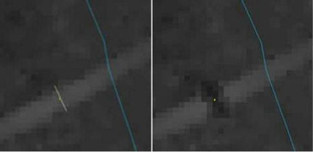
Figure 4. Before and after making channels at culvert locations using ArcHydro agree streams.

Figure 5. Location of culverts identified in LiDAR-DEM.
was used for the DEM reconditioning. The depth of culvert was used to recondition the DEM on the locations of the culverts through the ArcHydro DEM reconditioning function. Thus, the elevation at the culvert locations become accurate (lower than the elevations obtained from LiDAR data based DEM as LiDAR data cannot locate the culvert openings because they are buried below the roads).
The new DEM obtained after reconditioning for all culvert elevations was used to generate a new Turkey Creek watershed boundary and subwatersheds with ArcSWAT [20,37]. The automated watershed delineation processes of programs such as ArcSWAT [37] or BASINS model [38] use the Deterministic 8-neighbor (D8) algorithm for flow direction [39] based on the concept of steepest slope. Some of the documented weaknesses of D8-algorithm include tendency to generate parallel flow paths in flat areas, high sensitivity to inherent DEM errors, and inaccurate flow direction on convex slopes [40-42]. Other algorithms such as multiple flow direction (MFD), Deterministic-Infinity (D∞), Random-Eight Neighbor (Rho8), and Digital Elevation Model networks (DEMON) have been developed to address the above challenges [43]. This study does not address the effect of the algorithm used to automatically delineate watershed drainage area from DEM, but highlights the effects of DEM resolution using ArcSWAT which implements the D8 algorithm [39].
2.4. Hydrologic Analysis with Changed Watershed Boundary and Area
The historic stream flow data obtained by using the measured stage data and the stage-discharge relationship established in the early period [44] were archived in Forest Service data base [25]. No studies, however, were conducted or published using these flow data from this watershed for this period. The daily stream flow data was processed to obtain volume of water in cubic meters discharged in each year by multiplying by the drainage area with the given DEM method and conversion factors. The calculated mean annual outflow volume of 16.5 million cubic meters for the 13-year period was then divided by the calculated drainage area of the watershed obtained by each of the DEM methods since mid-1960’s to obtain the depth-based outflow. The 50-year (1951- 2000) average annual rainfall of 1370 mm obtained from the data collected at a nearby weather station at Santee Experimental Forest (SEF) headquarters was used to calculate the average annual runoff coefficient (ROC). The ROC is the ratio of average annual depth-based outflow (mm) and average annual rainfall (mm). The ROC was calculated to assess its uncertainty, for that matter the uncertainty of the overall average annual water balance of the watershed, due to uncertainty in drainage area obtained from each DEM type. The ROC calculated using the drainage area derived from the DEM based on the recent high resolution Li-DAR data was considered as a reference for compareson with the ROCs obtained using historic results.
3. Results and Discussion
3.1. Santee Experimental Forest
3.1.1. Detection of Historic Land Use Features
The LiDAR data were effective in delineating the drainage and agricultural water management features associated with the rice cultivation in the floodplain (Figure 6). The features range in size from dikes and dams (0.2 - 1.6 m height) to ditches (0.2 - 0.3 m depth). It’s important to note the prominence of these features on the watershed, and to realize that their occurrence is within a watershed that has a total relief of less than 4 m. Within the context of this landscape, these dikes and ditches are major topographic features. The only reflection of these historical agricultural water management features on the current USGS topographic map (scale 1:24,000) are the major impoundment structures (see Figure 1(b)), but only a few of those existing structures are denoted.
In a similar application, [15] used LiDAR data to map gullies and headwater streams under a forest canopy in South Carolina, and found that LiDAR data provided robust detection of small gullies and channels, except where they are narrow or parallel and closely spaced. They reported that the ability of LiDAR data to map gullies and channels in a forested landscape should improve channel network maps and topological models.
3.1.2. Effects of Historical Water Management Features on Watershed Hydrology
The historical water management features may have been
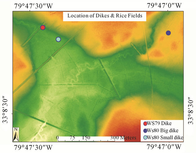
Figure 6. Depiction of surface topography derived from LiDAR data for a section of Huger Creek, Santee Experimental Forest. The location of dikes and ditches are noted.
affecting current watershed hydrology in several ways. Diversion ditches are affecting upland runoff processes including overland flow paths. These ditches were constructed to shunt water from reservoirs to fields located in the floodplain; hence they run perpendicular to the slope. The ditches, with the associated spoil bank, serve to interrupt surface runoff and to channel the runoff at points where water control structures existed (Figure 7).
The presence of these features is a major contradiction to the assumptions of hill slope runoff from the traditional resource data (topographic map). The effects of the collection and rechannelization are evident by drainage rivulets into the floodplain. The net effect of these ditches is to interrupt hillslope flow path, pool runoff, and redirect it through small channels. It is also likely that subsurface runoff is also affected. This may also ultimately alter travel time and time to peak of flooding at the watershed outlet.
The old field ditches and banks also affect runoff within the floodplain; these are major topographic features that will affect transport and routing, especially during flood stages. During non-flood periods, if the old ditches are not hydraulically linked to the stream, they may function as detention storage areas affecting infiltration positively and stream flow negatively.
3.1.3. Detection of Stream Network
The high resolution LiDAR data also proved useful in delineating the stream location. The USGS topographic maps convey a rather straight or direct-flowing stream; in contrast the stream generated with the LiDAR data illustrates a meandering channel (Figure 8).
As a result, the difference in stream channel configurations like the length and sinuosity among the two data sources is pronounced; for the stream reaches denoted in

Figure 7. LIDAR image showing a stream diversion ditch running parallel to the present channel. The ditch and associated berm interrupt surface runoff.
Figure 8, the total channel length from the USGS map is 1853 m and it is 2962 m from the LiDAR data (Table 2).
Sinuosity, a ratio of channel (thalweg) distance and downvalley distance, describes whether a channel is straight or meandering. The sinuosity values range from 1.0 for straight channels to as high as 4.0 for highly intricate meandering streams [45]. The calculated sinuosity values were also different for these reaches when calculated with the USGS and LiDAR stream data (Table 2). Both the length as well as sinuosity was not even detected for reaches R6 to R8 when the USGS map was used.
None of the stream reaches would be considered meandering with a sinuosity ratio of 1.5 or greater) when calculated from the USGS topographic map. In contrast two of the stream reaches (R2 and R3) actually meander, based on the sinuosity values > 1.5 calculated from the LiDAR data (Table 2). The 61% increase in channel length and recognition of sinuosity in some reaches has important ramifications when considering peak discharge, time to peak, routing, in-stream processes and pollutant export from these watersheds.
3.1.4. Changes in Hydrologic Functions
Water management structures that were devised for rice cultivation in the floodplain that began 300 years ago are affecting contemporary surface water hydrology and stream channel hydraulics. As a result, hydrologic and hydraulic functions of the watershed have been potentially altered from conditions that were presumed to exist in these now-forested watersheds (Table 3).
The changes are associated with alterations to hill slope runoff including its pathways, structures within the floodplain changing depressional storage, and increased channel length and flow routing which results in longer
Table 2. Stream length and sinuosity for segments identified in Figure 8.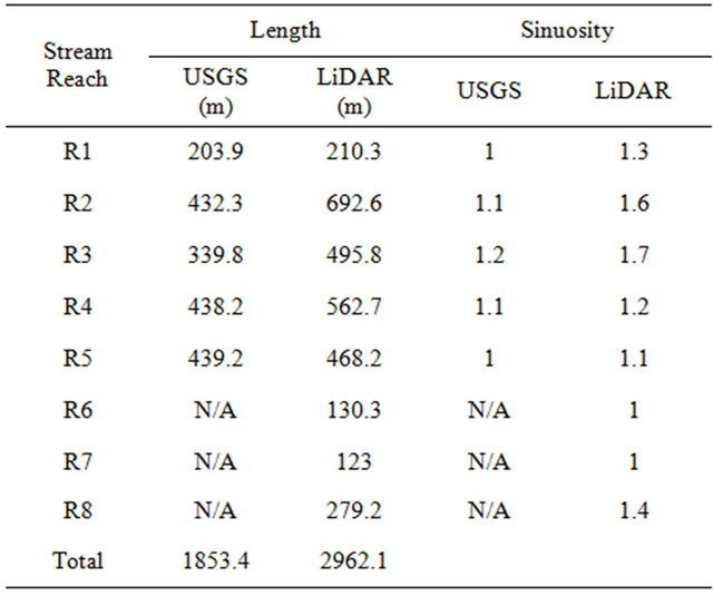
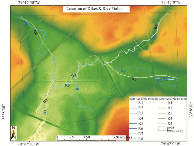
Figure 8. Overlay of the USGS topographic map (green) and LiDAR derived stream channel (blue).
Table 3. Effects of historical agricultural water management systems on hydrologic functions in floodplains of the Santee Experimental Forest.

time to peak and reduced peak runoff rate. While active water management structures increase surface depressional storage enhancing the wetland hydrologic functions (e.g., water table elevations and soil moisture), it is uncertain how these relic structures affect depressional storage since the control structures are not functional.
3.1.5. Implications for Modeling
When modeling hydrology on the SEF watershed, the landscape is represented by the readily available resource data (e.g., Figure 1). During model calibration, parameters and coefficients may be modified to achieve reasonable simulations, as compared to measured stream discharge. As an example, a common parameter to adjust for peak flow rates during calibration is the depressional storage, a parameter that is very difficult to measure directly [23]. It is evident that adjustments to depressional storage could mask or compensate for the effects of the actual channel and stream routing (Figure 8) and hill slope runoff (Figure 7). For example, depressional storage is a key parameter in the DRAINMOD model that controls the surface runoff rate after the soil is saturated and the surface storage is filled [46-48]. The effect is to modify the model behavior to achieve more accurate output, but if that calibration does not reflect actual hydrological processes, then the end results do not reflect accurately simulated processes within the watershed. Recently, [23] developed a GIS-based depressional storage capacity (DSC) model using USGS DEM data for one of the SEF watersheds (WS-77) and estimated 1 cm of effective depressional storage. When that storage factor was used to simulate stream discharge for the watershed using both DRAINMOD and its watershed-scale version, DRAINWAT [23,49], higher simulated peak flow rates were obtained for both the models for the 2003-2007 simulation period; that effect is likely due to an underestimation of the surface storage parameter for this watershed, which could result from not recognizing the historical water management structures not reflected in current DEMs.
3.2. Turkey Creek Watershed
3.2.1. Evolution of Drainage Areas
The watershed drainage area delineated in 1964 using the USGS topographic map with 1 inch = 2 miles scale is shown in Figure 9. Based on this the preliminary drainage area at that time was reported as 3240 ha (8000 ac) [44]. Some of the boundary followed the existing road. This drainage area resulted in the average annual ROC of 0.38 (Table 1). Such a value is generally observed for mountainous upland conditions [50] and is considered high for predominantly forested low-gradient watersheds in the humid coastal region [5,50].
The second estimated drainage area of the Turkey creek watershed in early 1970s was based on the USGS topographic map of 1 inch = 1 mile scale (Figure 10, Table 1).
The area of the watershed using this map was estimated at 4575 ha (11,300 acres) [51], which was about 41% higher than the initial estimate of 3240 ha. As a result, the calculated average annual ROC for this DEM was 0.27 only (Table 1), which is in the range of values obtained for similar coastal forested watersheds [52].
Later when the watershed gauging station was revitalized in late 2004 for conducting multi-collaborative hydrologic studies on this and adjacent 1st and 2nd order watersheds, a need of more reliable drainage area estimate was perceived. Accordingly, the new DEMs with 30 m horizontal and 1 m vertical resolution available in 2004 from SCDNR were used to delineate the watershed using the ArcView GIS software tools (Figure 11).
The new watershed boundary shown in Figure 11 yielded the drainage area approximately at 4920 ha (12,150 acres) (Table 1). This was an increase of 7.5% compared to the estimate and a 52% increase from the initial (1964) estimate. Thus the drainage area continued to increase. Accordingly, the calculated average annual ROC continued to decrease to 0.25 (Table 1), which is also in the range of published data for this type of coastal forested watersheds [50,52,53]. Amatya and Radecki-Pawlik [25] used these data to compare the streamflow dynamics of this watershed with the two adjacent 1st and 2nd order watersheds. No field verification was done.
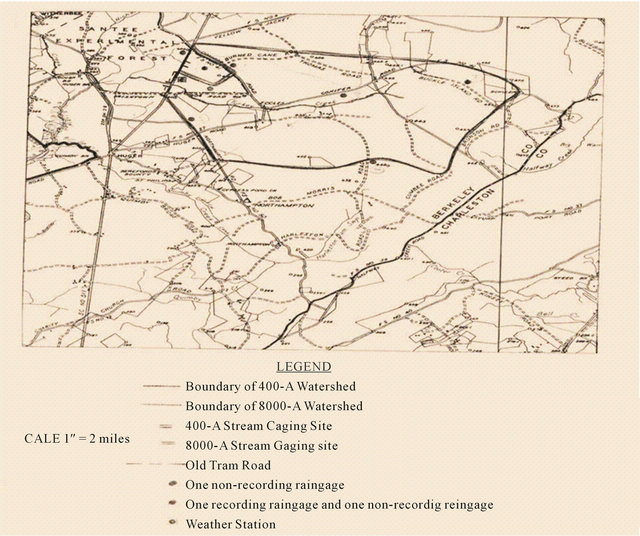
Figure 9. Watershed boundary using 1” = 2 mile USGS topographic map.
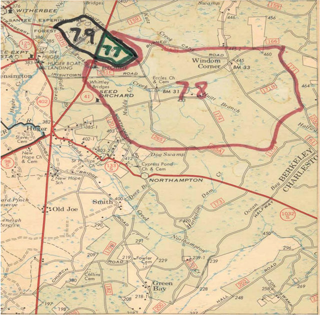
Figure 10. Watershed boundary using 1” = 1 mile USGS topographic map.

Figure 11. Watershed boundary using 30 m horizontal and 1 m vertical resolution DEM (SCDNR, 2004).
Later in 2005 USGS obtained an estimate of 5880 ha (14,520 acres) as the drainage area at the outlet of the current gauging station (Table 1, Figure 12, green color) using the SC 14-digit HUC with the 1:24,000-scale 7.5- minute series topographic maps as the source maps and 1:100,000-scale Digital Line Graphs as base maps [27]. This was still a 19.5% increase from the previous SCDNR2004 based DEM result. No field checking for road boundaries as well as cross drainage structures like culverts was done for this estimate although these may have dramatic effects on the reconditioned DEMs and the derived drainage area. Accordingly, the average annual ROC was found to be 0.21 for this area (Table 1), which is also in the range of the published data for the coastal forested watersheds [50,52,53].
In 2006, new DEMs obtained from the USGS Enhanced 1:24,000 true 10 m horizontal 1 m vertical DEM became available to update the watershed boundary. In this case the SWAT interface in ArcView [37] was used to delineate the watershed as shown in Figure 13. The delineation also considered the drainage pathways due to forest roads and 44 culverts surveyed during the 2006- 2007 period [28]. The ArcView SWAT delineation yielded the highest drainage area of 7260 ha (Table 1). This was 124% higher than the initial estimate of 3240 ha and 47.6% higher than the estimate using the 30 m × 30 m DEM. This was possibly due to errors in the 10 m enhanced DEM as reported recently by [11].
This new drainage area resulted in the lowest average annual ROC value of 0.17 (Table 1). Ongoing studies on the Turkey Creek watershed at that time used this drainage area to calculate the new depth-based outflow in estimating field water balance [2], assessing the rainfallrunoff storm event dynamics [5], as well as validating a SWAT model [1,28].
Later in 2010 using partial LiDAR dataset for the
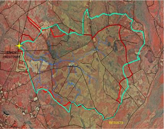
Figure 12. Watershed boundary using SC14-digitHUC (green) overlaid on SCDNR2005 boundary (red).
small lower part of the Turkey Creek watershed, which is within the Santee Experimental Forest, a new drainage area of 6,510 ha was calculated, which was 10.3% lower than the ArcView/SWAT computed area of 7260 ha and 10.7% higher than the SC 14-digit HUC generated area of 5980 ha. The average annual ROC was 0.19 based on this area of 6510 ha (Table 1) and is lower compared to similar coastal watersheds.
Finally, in 2011 the most updated high resolution 1.5 m × 1.5 m and 0.18 m vertical resolution DEM based on the complete LiDAR data for the watershed was used to redefine the boundary and corresponding area using the ArcSWAT model as shown in blue color in Figure 14. The area calculated by this method as a reference was 5240 ha with a corresponding calculated average annual ROC of 0.24 (Table 1), which was very close to the similar other forested watersheds in the coastal plain [50,52,53]. The area of only 5240 ha estimated using the Li-DAR-based DEM is about 6.5% higher than the previously estimated area of 4920 ha by SCDNR2004 method, indicating that the 30 m × 30 m horizontal and 1 m vertical resolution DEM was well within the water balance errors [18]. The USGS defined drainage area of 5880 ha based on 14-digit HUC was 12.2% higher than this LiDAR-based DEM as a reference.
Interestingly, if the areas that were drained by the road culverts (based on DEM reconditioning and field verifycation) outside of the watershed boundary are not considered (or included as if there were no culverts) the LiDAR-based DEM (brown color) also provides exactly the same drainage area (5880 ha) as the one obtained by using the 2011-USGS 14-digit HUC data. This indicates that for areas without culverts the DEM based on the 14- digit HUC may be as accurate as the LiDAR based DEM for these LCP watersheds. However, further analysis of more LCP watersheds is needed to definitively confirm this observation.
Data in Figure 15 shows the uncertainty in average annual runoff coefficients as a result of variability in the corresponding estimated drainage areas of the Turkey Creek watershed for various DEM types used since 1960’s. Clearly, a highest ROC of 0.38 was obtained for the lowest area estimated using very first initial USGS topographic map of 1” = 2 mi scale in 1960’s. The lowest ROC of 0.17 was obtained for the largest estimated area of 7260 ha by using ArcSWAT delineation with the 1:24,000-scale true 10 m horizontal and 1 m vertical resolution DEMs. We believe both of these DEMs produced larger errors in estimating average annual ROCs, as a result of errors in drainage areas.
The drainage area of 4920 ha calculated using 30 m DEM from SCDNR in 2004 was the closest, with only about 6% underestimate, to the area of 5240 ha obtained by the LiDAR data in 2011. However, the historic 1969
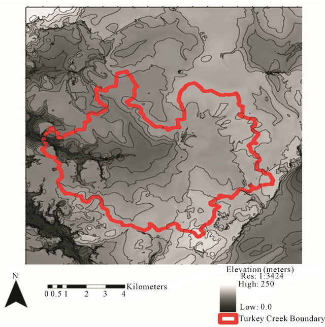
Figure 13. Watershed boundary using 2005 USGS enhanced 1:24,000 scale 10 m × 10 m and 1 m vertical DEM.
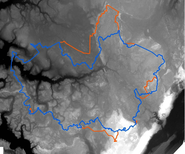
Figure 14. Watershed boundary using 1.5 m horizontal and 0.18 m vertical resolution DEM from the 2011 LiDAR data (Blue color with and brown color without accounting for culverts).
1” = 1 mi topographic map based area of 4575 ha was 12.6% lower than the LiDAR-based estimate. These results are consistent with those by the NOAA’s Office of Hydrologic Development [54] who reported a reduction of errors in basin area estimates by more than half by
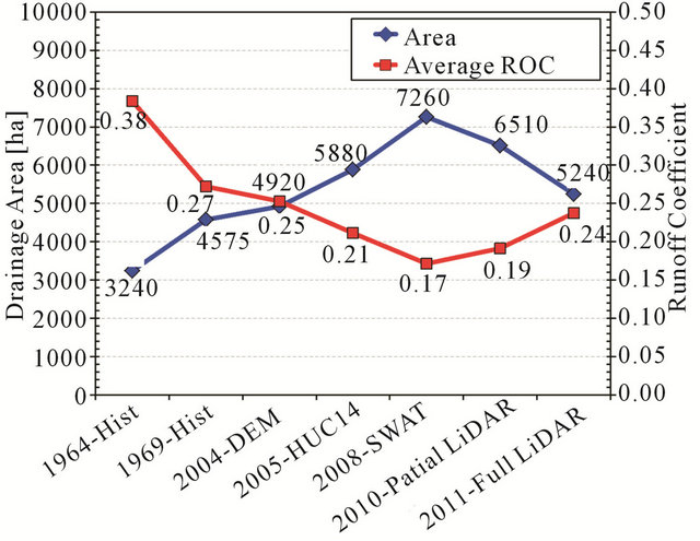
Figure 15. Estimated drainage areas of the Turkey Creek watershed using various DEM types and the corresponding average annual runoff coefficients.
using 30 m DEM compared to the 400 m DEMs for mild to moderate sloped watersheds with less than 78 km2 area in the states of Oklahoma and Kansas.
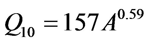
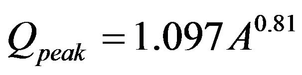
The effects of uncertainty in drainage areas obtained by various DEM types can be propagated in many hydrologic studies including water and nutrient balances, spatially distributed modeling (SWAT, MIKESHE, HSPF, DRAINWAT, WEPP, etc.) and engineering designs for water resources structures involving Rational Method (Equation (1)), USGS regional flood discharge formula (Equation (2)) [55], peak discharge estimates (Equation (3)) [56], pollutant export coefficients, estimating flow rates using empirical approaches for ungauged basins (Equation (4)) [57], designing the best management practices, and nutrient loading estimates (Equation (5)) [58,59] generally used in Total Maximum Daily Load (TMDL) developments.
 (1)
(1)
 (2)
(2)
 (3)
(3)
 (4)
(4)
 (5)
(5)
where Qpeak is the peak discharge, C is a runoff coefficient, I is rainfall intensity, A is field or drainage area, Q10 is peak discharge with a return period of 10 years, Qp is long-term daily flow exceeded p% of the time, [a, b, c, d, and e] are regional coefficients, X1 and X2 are watershed descriptors, Lio is a nutrient loading at a field edge, and Lec is the average export coefficient for a given land management practice (soil, crop/vegetation, and water management).
While the importance of high resolution LiDAR-based DEM for delineation of accurate drainage areas was demonstrated, it may have other applications also as shown by [30] for the Santee Experimental Forest. The authors reported that improvements in hydrologic functions and pathways used in hydrologic models and assessments can be achieved by using these high resolution DEMs that are capable of identifying the remnants of legacy water management structures left from rice planting in 1700’s in the SC Lower Coastal Plain, which otherwise were not identified using the regular and enhanced DEMs. Similarly, [23] used DEM-based approach including LiDAR data to quantify the surface storage parameter widely used in hydrologic models for predicting the peak flow rates. Lang and McCarty [17] demonstrated the ability of LiDAR intensity data for forest inundation mapping on forested wetlands in eastern shore of Maryland. Eeckhaut et al. [36] concluded that LiDAR data enabled experts to find ten new landslides and to correct the boundaries of 11 of the 77 landslides mapped during the field survey. Our work here used recent high density LiDAR data with field verification to identify more culverts in the stream tributary network than possible using the NHD dataset. Our findings are consistent with recent findings of [60], who reported that stream datasets derived from semi-automated and automated interpretation of LiDAR derived DEMs were considerably more accurate than NHD high resolution and Plus datasets. These authors found that LiDAR derived datasets significantly increased percent area and total number of wetlands that were considered connected.
4. Summary and Conclusions
There is a tremendous need to accurately represent environmental processes on the landscape. Questions involving climate change, land use effects, urbanization, etc., require a thorough understanding of the processes regulated by hydrology because the consequential thresholds are usually small. While models are the principal tools for conducting assessments, representations from spatially distributed, physically-based models are only as effective as the mathematical representation of the processes and the accuracy and resolution of the supporting data. We have shown that historical land use features may affect contemporary watershed hydrologic and transport processes, to illustrate that the modeling process (e.g., calibration) may compensate for inherent features in the landscape. Adoption of higher resolution data, whenever available, will challenge and ultimately improve our understanding of hydrologic and pollutant cycling processes and hence model applications [10,12- 15,17,60]. With the improvement in computer processing speed, sensor technology, and advanced models, high resolution data are being analyzed on a faster scale and providing better and efficient results. In areas where water resources are critical and existing data relatively poor (e.g., coastal plain), acquisition of high resolution topographic data will greatly enhance our ability to assess hydrologic functions including water, nutrient and carbon balances.
DEMs based on high resolution topographic data such as LiDAR with field verification for cross drainage structures and roadbeds of the study watershed should be used for estimating more reliable boundary/drainage areas often used in hydrologic studies in the flat, low-gradient coastal plain landscapes. The area delineated by using the 14-digit HUC may be as accurate as the one obtained by the LiDAR-based DEM for these LCP watersheds as long there are no roads or culverts on the landscape. The drainage area estimated using the classical 30 m horizontal and 1 m vertical resolution DEM was found to be much more accurate than the USGS enhanced 1:24,000 true 10 m horizontal 1 m vertical DEM when compared to the LiDAR-based DEM in this study. Although the high resolution LiDAR-based DEM was considered as the most accurate for use as a reference in this study, we should still acknowledge some uncertainties and errors in the LiDAR data processing also as various software used to process them have some limitations and potential errors (e.g., errors due to inherent structure of algorithms for automatic watershed delineation).
5. Acknowledgements
The authors would like to acknowledge the USDA Forest Service Southern Research Station Civil Rights Committee Summer Student Hire Program for supporting a part of this study using the LiDAR data and field verification works by Jose Martin, the former student at Gainesville State College. We also would like to thank Dr. Jim Scurry at SC Department of Natural Resources for providing the much needed LiDAR data (draft), Beth Haley, former student of College of Charleston for field survey of culverts and processing the 2005 enhanced DEM data, Lisa Wilson, former student of College of Charleston for processing the SCDNR2005 data, Andy Harrison, Hydrologic Technician at Forest Service in Cordesville, SC for various levels of support in field/data, and TetraTech for digitizing the historic streamflow data used in this study. Bill Hansen, Forest Hydrologist, at Francis Marion & Sumter National Forests office, SC are also acknowledged for their advice and suggestions on DEM data.
REFERENCES
- D. M. Amatya and M. K. Jha, “Evaluating the Swat Model for a Low-Gradient Forested Watershed in Coastal South Carolina,” Transactions of the ASABE, Vol. 54, No. 6, 2011, pp. 2151-2163.
- D. M. Amatya, T. J. Callahan, C. Trettin and A. Radecki- Pawlik, “Hydrologic and Water Quality Monitoring on Turkey Creek Watershed, Francis Marion National Forest, SC,” ASABE Annual International Meeting, Reno, 2009, pp. 21-24.
- D. Bosch, J. Sheridan and F. Davis, “Rainfall Characteristics and Spatial Correlation for the Georgia Coastal Plain,” Transactions of the ASAE, Vol. 42, No. 6, 1999, pp. 1637-1644.
- C. G. Garrett, V. M. Vulava, T. J. Callahan and M. L. Jones, “Groundwater-Surface Water Interactions in a Lowland Watershed: Source Contribution to Stream Flow,” Hydrological Processes, Vol. 26, No. 21, 2012, pp. 3195-3206. doi:10.1002/hyp.8257
- I. B. La Torre Torres, D. M. Amatya, G. Sun and T. J. Callahan, “Seasonal Rainfall-Runoff Relationships in a Lowland Forested Watershed in the Southeastern USA,” Hydrological Processes, Vol. 25, No. 13, 2011, pp. 2032- 2045. doi:10.1002/hyp.7955
- T. M. Williams, D. M. Amatya, D. R. Hitchcock and A. E. Edwards, “Streamflow and Nutrients from a Karst Watershed with a Downstream Embayment: Chapel Branch Creek,” In Press, ASCE Journal of Hydrologic Engineering, Posted Ahead of Print January 26, 2013.
- T. J. Callahan, V. M. Vulava, M. C. Passarello and C. G. Garrett, “Estimating Groundwater Recharge in Lowland Watersheds,” Hydrological Processes, Vol. 26, No. 19, 2012, pp. 2845-2855. doi:10.1002/hyp.8356
- D. M. Amatya, M.K. Jha, A. E. Edwards, T. M. Williams, and D. R. Hitchcock, “SWAT-Based Streamflow and Embayment Modeling of a Karst affected Chapel Branch Watershed, SC,” Transaction of the ASABE, Vol. 54, No. 4, 2011, pp. 11311-1323
- Z. Dai, C. C. Trettin, C. Li, H. Li, G. Sun and D. M. Amatya, “Effect of Assessment Scale on Spatial and Temporal Variations in CH4, CO2 and N2O Fluxes in a Forested Wetland,” Water, Air, & Soil Pollution, Vol. 223, No. 1, 2012, pp. 253-265. doi:10.1007/s11270-011-0855-0
- P. C. Beeson, A. M. Sadeghi, M. W. Lang, M. D. Tomer and C. S. T. Daughtry, “Sediment Delivery Estimates in Water Quality Models Altered by Resolution and Source of Topographic Data,” Journal of Environmental Quality, 2013. doi:10.2134/jeq2012.0148
- S. S. Panda, K. Burry and C. Tamblyn, “Wetland Change and Cause Recognition in Georgia Coastal Plain,” ASABE International Conference, Dallas, 2012.
- C. S. Renschler and D. C. Flanagan, “Site-Specific Decision-Making Based on RTK GPS Survey and Six Altaernative Elevation Data Sources: Soil Erosion Predictions,” Transactions of the ASAE, Vol. 51, No. 2, 2008, pp. 413- 424.
- A. A. Aziz, B. L. Steward, A. Kaleita and M. Karkee, “Assessing the Effects of DEM Uncertainty on Erosion rate Estimation in an Agricultural Field,” Transactions of the ASABE, Vol. 55, No. 3, 2012, pp. 785-798.
- R. L. Perroy, B. Bookhagen, G. P. Asner and O. A. Chadwick, “Comparison of Gully Erosion Estimates Using Airborne and Ground-Based LiDAR on Santa Cruz Island, California,” Geomorphology, Vol. 118, No. 3-4, 2010, pp. 288-300. doi:10.1016/j.geomorph.2010.01.009
- L. A. James, D. G. Watson and W. F. Hansen, “Using LiDAR Data to Map Gullies and Headwater Streams under Forest Canopy: South Carolina, USA,” Catena, Vol. 71, No. 1, 2007, pp. 132-144. doi:10.1016/j.catena.2006.10.010
- S. P. Wechsler, “Uncertainties Associated with Digital Elevation Models for Hydrologic Applications: A Review,” Hydrology and Earth System Sciences Discussions, Vol. 11, No. 4, 2007, pp. 1481-1500. doi:10.5194/hess-11-1481-2007
- M. W. Lang and G. W. McCarty, “LiDAR Intensity for Improved Detection of Inundation below the Forest Canopy,” Wetlands, Vol. 29, No. 4, 2009, pp. 1166-1178. doi:10.1672/08-197.1
- S. V. Harder, D. M. Amatya, T. J. Callahan, C. C. Trettin and J. Hakkila, “Hydrology and Water Budget for a Forested Atlantic Coastal Plain Watershed, South Carolina,” JAWRA Journal of the American Water Resources Association, Vol. 43, No. 3, 2007, pp. 563-575. doi:10.1111/j.1752-1688.2007.00035.x
- B. Ambroise, J. L. Perrin and D. Reutenauer, “Multi- Criterion Validation of a Semi-Distributed Conceptual Model of the Water Cycle in the Fecht Catchment (Vosges Massif, France),” Water Resources Research, Vol. 31, No. 6, 1995, pp. 1467-1481. doi:10.1029/94WR03293
- J. G. Arnold, R. Srinivasan, R. S. Muttiah and J. Williams, “Large Area Hydrologic Modeling and Assessment Part I: Model Development,” JAWRA Journal of the American Water Resources Association, Vol. 34, No. 1, 2007, pp. 73-89. doi:10.1111/j.1752-1688.1998.tb05961.x
- Z. Dai, C. Li, C. Trettin, G. Sun, D. Amatya and H. Li, “Bi-Criteria Evaluation of the MIKE SHE Model for a Forested Watershed on the South Carolina Coastal Plain,” Hydrology and Earth System Sciences, Vol. 14, No. 6, 2010, pp. 1033-1046. doi:10.5194/hess-14-1033-2010
- S. B. Hilliard, “Antebellum Tidewater Rice Culture in South Carolina and Georgia,” In: J. R. Gibson, Ed., European Settlement and Developmentin North America, University of Toronto Press, Toronto, 1978, pp. 91-115.
- J. K. O. Amoah, D. M. Amatya and S. Nnaji, “Quantifying Watershed Surface Depression Storage: Determination and Application in a Hydrologic Model,” HYDROLOGICAL PROCESSESHydrol. Process, Wiley Online Library, 2012. wileyonlinelibrary.com
- PhotoScience, “Airborne Laser Terrain Mapping for Santee Experimental Forest, SC. Photo Science Geospatial Solutions,” Lexington, 2007.
- D. M. Amatya and A. Radecki-Pawlik, “Flow Dynamics of Three Experimental Forested Watersheds in Coastal South Carolina (USA),” ACTA Scientiarum Polonorum, Formatio Circumiectus, Vol. 6, No. 2, 2007, pp. 3-17.
- D. E. Bower, C. Lowry, M. A. Lowery and N. M. Hurley, “USGS Water Resources Investigations Report WRIR 99-4015,” 1999. http://sc.water.usgs.gov/publications/abstracts/wrir99-4015.html
- J. P. Eidson, C. M. Lacy, L. Nance, W. F. Hansen, M. A. Lowery and N. M. Hurley, Jr., “Development of a 10- and 12-Digit Hydrologic Unit Code Numbering System for South Carolina, 2005,” 2005.
- E. B. Haley, “Field Measurements and Hydrologic Modeling of the Turkey Creek Watershed, South Carolina (SC),” Master’s Thesis, Graduate School of the College of Charleston, Charleston, 2007.
- DeLorme, “A Topographic Map Software,” 2002. www.delorme.com
- C. C. Trettin, D. M. Amatya, C. Kaufman, N. Levine and R. T. Morgan, “Recognizing Change in Hydrologic Functions and Pathways due to Historical Agricultural Use—Implications to Hydrologic Assessments and Modeling,” The Third Interagency Conference on Research in the Watersheds, Estes Park, 8-11 September 2008, 5 p.
- J. Scurry, “Raw LiDAR Data for Berkeley County, SC, SCDNR,” 2011.
- A. Imagery, “Quick Terrain Modeler (QTM),” Version 7.1.5, 2012.
- D. Civco, “ERDAS IMAGINE Remote-Sensing, Image- Processing and GIS Software,” Photogrammetric Engineering and Remote Sensing, Vol. 60, No. 1, 1994, pp. 35-39.
- ESRI, “ESRI ArcGIS,” Version 9.3.1., Redlands, 2009.
- J. D. Simley and W. J. Carswell, Jr., “The National Map—Hydrography,” US Geological Survey Fact Sheet, Vol. 3054, No. 1, 2009, 4 p.
- M. Eeckhaut, J. Poesen, G. Verstraeten, V. Vanacker, J. Nyssen, J. Moeyersons, et al., “Use of LIDAR-Derived Images for Mapping Old Landslides under Forest,” Earth Surface Processes and Landforms, Vol. 32, No. 5, 2006, pp. 754-769. doi:10.1002/esp.1417
- M. D. Di Luzio, R. Srinivasan, J. G. Arnold and S. L. Neitsch, “Arcview Interface for SWAT2000: User’s Guide- (2002),” 12 December 2012. http://www.brc.tamus.edu/swat/downloads/doc/swatav2000.pdf
- R. S. Kinerson, J. L. Kittle and P. B. Duda, “BASINS: Better Assessment Science Integrating Point and Nonpoint Sources,” In: Decision Support Systems for Risk-Based Management of Contaminated Sites, A. Marcomini, G. W. Suter II and A. Critto, Eds., Springer, 2009, pp. 1-24.
- J. F. O’Callaghan and D. M. Mark, “The Extraction of Drainage Networks from Digital Elevation Data,” Computer Vision, Graphics, and Image Processing, Vol. 28, No. 3, 1984, pp. 323-344. doi:10.1016/S0734-189X(84)80011-0
- R. Jones, “Algorithms for Using a DEM for Mapping Catchment Areas of Stream Sediment Samples,” Computers & Geosciences, Vol. 28, No. 9, 2002, pp. 1051-1060. doi:10.1016/S0098-3004(02)00022-5
- A. R. Paz, W. Collischonn, A. Risso and C. A. B. Mendes, “Errors in River Lengths Derived from Raster Digital Elevation Models,” Computers & Geosciences, Vol. 34, No. 11, 2008, pp. 1584-1596. doi:10.1016/j.cageo.2007.10.009
- J. P. Wilson, C. S. Lam and Y. Deng, “Comparison of the Performance of Flow-Routing Algorithms Used in GIS- Based Hydrologic Analysis,” Hydrological Processes, Vol. 21, No. 8, 2007, pp. 1026-1044. doi:10.1002/hyp.6277
- K. M. Crombez, “Comparing Flow Routing Algorithms for Digital Elevation Models,” Digital Terrain Analysis (Geo428), Project Paper for Michigan State University, 2008, pp. 1-9.
- C. E. Young, “Precipitation-Runoff Relations on Small Forested Watersheds in the Coastal Plain. Study Plan Addendum No. 2,” USDA Forest Service Technical Report FS-SE-1602, 1965.
- N. D. Gordon, T. A. McMahon, B. L. Finlayson, C. J. Gippel and R. J. Nathan, “Stream Hydrology: An Introduction for Ecologists,” Wiley, Hoboken, 2004.
- P. Haan and R. Skaggs, “Effect of Parameter Uncertainty on DRAINMOD Predictions: I. Hydrology and Yield,” Transactions of the ASAE, Vol. 46, No. 4, 2003, pp. 1061- 1067.
- K. Konyha and R. Skaggs, “A Coupled, Field Hydrology: Open Channel Flow Model: Theory,” Transactions of the ASAE, Vol. 35, No. 5, 1992, pp. 1431-1440.
- R. Skaggs, “A Water Management Model for Shallow Water Table Soils,” Technical Report No. 134, North Carolina State University, Water Resources Research Institute of the University of North Carolina, Raleigh, 1978.
- J. Amoah, “A New Methodology for Estimating Watershed-Scale Depression Storage,” Ph.D. Dissertation, Department of Civil & Environmental Engineering, Florida A&M University, Tallahassee, 2008, 202 p.
- G. Sun, S. G. McNulty, D. M. Amatya, R. W. Skaggs, L. W. Swift, J. P. Shepard, et al., “A Comparison of the Watershed Hydrology of Coastal Forested Wetlands and the Mountainous Uplands in the Southern US,” Journal of Hydrology, Vol. 263, No. 1-4, 2002, pp. 92-104. doi:10.1016/S0022-1694(02)00064-1
- S. Laseter, “Stage-Flow Fortran Programs for Processing Discharge Data for Santee Experimental Forest Watersheds,” USDA Forest Service, Coweeta Hydrologic Laboratory, Otto, 2008.
- D. Amatya, M. Miwa, C. Harrison, C. Trettin and G. Sun, “Hydrology and Water Quality of Two First Order Forested Watersheds in Coastal South Carolina,” In: ASABE Annual International Meeting, Portland, 9-12 July 2006, 22 p.
- G. M. Chescheir, M. E. Lebo, D. M. Amatya, J. Hughes, J. W. Gilliam and R. W. Skaggs, “Hydrology and Water Quality of Forested Lands in Eastern North Carolina,” Tech Bullet 320, North Carolina State University, Raleigh, 2008, 79 p.
- OHD, “Basin Delineation with a 400 m Terrain Dataset,” 2011. http://www.nws.noaa.gov/oh/hrl/gis/delineation.html
- W. B. Guimaraes and L. R. Bohman, “Techniques for Estimating Magnitude and Frequency of Floods in South Carolina,” USGS Water-Resources Investigations Report, 1992, pp. 91-4157.
- J. M. Sheridan, “Peak Flow Estimates for Coastal Plain Watersheds,” Transactions of the ASAE, Vol. 45, No. 5, 2002, pp. 1319-1326.
- H. S. Ssegane, D. M. Amatya, E. W. Tollner, Z. Dai and J. E. Nettles, “Estimation of Daily Streamflow of Southeastern Coastal Plain Watersheds by Combining Estimated Magnitude and Sequence (Tentatively Accepted),” Journal of the American Water Resources Association, In Press, 2013, pp. 1-17.
- D. M. Amatya, G. M. Chescheir, G. P. Fernandez, R. W. Skaggs, F. Birgand and J. Gilliam, “Lumped Parameter Models for Predicting Nitrogen Transport in Lower Coastal Plain Watersheds,” Report No. 347, North Carolina Water Resources Research Institute, Raleigh, 2003.
- M. Beaulac and K. Reckhow, “An Examination of Land Use-Nutrient Export Relationships,” Journal of the American Water Resources Bulletin, Vol. 18, No. 6, 1982, pp. 1013-1024.
- [61] M. Lang, O. McDonough, G. McCarty, R. Oesterling and B. Wilen, “Enhanced Detection of Wetland-Stream Connectivity Using LiDAR,” Wetlands, Vol. 32, No. 3, 2012, pp. 461-473.