Natural Science
Vol.5 No.5A(2013), Article ID:32013,13 pages DOI:10.4236/ns.2013.55A007
Habitat protection for sensitive species: Balancing species requirements and human constraints using bioindicators as examples
![]()
1Division of Life Sciences, Rutgers University, Piscataway, NJ, USA; *Corresponding Author: burger@biology.rutgers.edu 2Environmental and Occupational Health Sciences Institute, Rutgers University, Piscataway, NJ, USA 3Consortium for Risk Evaluation with Stakeholder Participation, Vanderbilt University, Nashville, TN, USA 4Environmental and Occupational Medicine, UMDNJ-Robert Wood Johnson Medical School, Piscataway, NJ, USA 5Department of Civil and Environmental Engineering, Vanderbilt University, Nashville, TN, USA 6Conserve Wildlife Foundation of New Jersey, Greenwich, NJ, USA 7Herpetological Associates Inc., Jackson, NJ, USA 8Ecology and Evolution Graduate Program, Rutgers University, New Brunswick, NJ, USA
Copyright © 2013 Joanna Burger et al. This is an open access article distributed under the Creative Commons Attribution License, which permits unrestricted use, distribution, and reproduction in any medium, provided the original work is properly cited.
Received 26 February 2013; revised 28 March 2013; accepted 10 April 2013
Keywords: Assessment; Environmental Monitoring; Bioindicators; Habitat vulnerabilities; Salmon; Frog; Snake; Bird
ABSTRACT
Vertebrates have particular habitat needs as a function of life cycle and reproductive stage. This paper uses four species as examples to illustrate a paradigm of environmental assessment that includes physical, biological, toxicological and human dimensions. Species used include Chinook salmon (Oncorhynchus tshawytscha), northern leopard frog (Rana pipiens), northern pine snake (Pituophis m. melanoleucus), and red knot (Calidris canutus rufa, a sandpiper). The life cycles of these species include reliance on habitats that are aquatic, terrestrial, aerial, or combinations of these. Two species (frog, snake) are sedentary and two (salmon, sandpiper) are long-distance migrants. While some measurement endpoints are similar for all species (reproductive success, longevity, contaminant loads), others vary depending upon life cycle and habitat. Salmon have a restricted breeding habitat requiring coarse sand, moderate current, and high oxygen levels for adequate egg incubation. Leopard frogs require still water of appropriate temperature for development of eggs. Pine snakes require sand compaction sufficient to sustain a nest burrow without collapsing, and full sun penetration to the sand to allow their eggs in underground nests to incubate and hatch. Red knots migrate to high Arctic tundra, but incubate their own eggs, so temperature is less of a constraint, but feedinging habitat is. These habitat differences suggest the measurement endpoints that are essential to assess habitat suitability and to manage habitats to achieve stable and sustainable populations. Habitat use and population stability have implications for human activities for some, but not all species. Salmon are important economically, recreationally, and as part of Native American culture and diet. Red knots are of interest to people mainly because of their long, intercontinental migrations and declining populations. Other measurement endpoints for these four species illustrate the differences and similarities in metrics necessary to assess habitat needs. The implications of these differences are discussed.
1. INTRODUCTION
All animals have specific habitat requirements that contribute to their survival and reproductive success, and these requirements shift at different times of their life cycle. Some species, termed eurytopic, have broad habitat tolerance (e.g. for salinity, temperature), while others have narrow constraints (stenotopic). The habitat required for breeding may be different from habitat used at other times of the year, habitat needs may differ at different developmental stages or ages, or habitat use may vary as a function of habitat suitability. Cultural aspects are often ignored in environmental monitoring plans and assessments, but the roles that human society, values and perceptions play in both environmental monitoring and environmental management are increasingly important [1]. Many books and refereed papers discuss environmental assessment, monitoring, bioindicators, biomarkers, sustainability, and risk [2,3]. The importance of human dimensions on environmental well-being and on population stability has been recognized [1], but the biological aspects of monitoring, traditional environmental assessment, and human dimensions have seldom been combined [4,5]. Examining different levels of assessment of habitat may be necessary to understand the status and trends for species, particularly those that are endangered, threatened, or of special concern.
In this paper, we use four bioindicator species to examine the levels of assessment and the types of measures or biomarkers that can be used for assessment. The species considered, selected to represent different life cycles and types of habitat requirements, include Chinook salmon (Oncorhynchus tshawytscha), northern leopard frog (Rana pipiens), northern pine snake (Pituophis m. melanoleucus), and red knot (Calidris canutus rufa). We were especially interested in the measurement endpoints (or biomarkers) that could be used to assess overall habitat needs, with the assessment endpoint being the maintenance of species that are considered of “special concern”, “threatened” or “endangered”. Assessing the health and well-being of animal populations is an important aspect of environmental management. There are several levels of environmental assessment that should be considered when protecting habitat for species of special concern, whether endangered or not. The levels of assessment that we believe are important are: 1) physical; 2) ecological; 3) ecotoxicology; 4) human health; and 5) sustainability, and a combination thereof.
2. APPROACH
Our overall approach is to: 1) describe briefly the life history, geographical range, habitat needs, human constraints, and key conservation issues for each bioindicator; 2) enumerate the types of biomarkers that can be used to examine habitat; and 3) propose the types of measurement endpoints or biomarkers that can be used for the four bioindicator species. Our selection of bioindicator species reflects different lifestyles, life cycles, habitat use, and migration patterns. Chinook salmon that run up the Columbia River in the spring to spawn in the Snake River are federally endangered, but the much larger “fall run” population is not endangered [6]. Northern pine snakes are endangered or threatened in most states where they occur, and red knot is a candidate species for federal listing. The widespread northern leopard frog is collected for research, education, bait, and food in many northern states and Canada. The complexities of life cycles results in different measurement endpoints to assess habitat quality with the assessment paradigm. Information is generally from the published literature, although human dimensions, key conservation issues, and measurement endpoints are derived from life history data and our own collective experience with these species. In this paper, bioindicator refers to the species, and measurement endpoint or biomarker refers to the characteristic that can be measured for bioindicator.
3. BIOINDICATOR EXAMPLES
General life history characteristics, ranges, habitat requirements, human dimensions, conservation issues, and possible mitigations to maintain healthy populations are given in Table 1. The paradigm for assessment (physical, ecological, ecotoxicological, human health/human dimensions, and sustainability), with examples, is given in Table 2. This paradigm can be used for other species. Together with information provided in Tables 1 and 3 for specific biomarkers, scientists, conservationists, managers, public policy makers and the general public can make decisions about designing assessment and biomonitoring plans, remediation and restoration, and long-term management of habitat for sustainable populations. It is not our intent to provide complete life histories, but rather to provide enough information that is relevant for understanding habitat constraints. Only with specific measurement endpoints can spatial and temporal trends be determined.
3.1. Chinook Salmon
Salmon are anadromous, laying their eggs in freshwater, migrating to the sea as juveniles, and returning years later as mature adults to breed. There is controversy about salmon taxonomy, including genetic lineages of the same species [7]. Salmon are heavily fished both recreationally and commercially, as well as being culturally important to Native Americans [8]. In the Columbia River, there are five species of salmon [9], and some populations or lineages are threatened or endangered [6]. The Hanford Reach (adjacent to the Department of Energy’s Hanford Site), is the most significant spawning habitat for fall Chinook salmon [10]. Historically, fall Chinook salmon spawned over a 900 km distance of the Columbia River, but because of dams and disturbance, they are now largely restricted to a 90 km section of the Hanford Reach [11].
Salmon conservation in the Pacific Northwest is complicated by the hydroelectric system of dams [12], har-
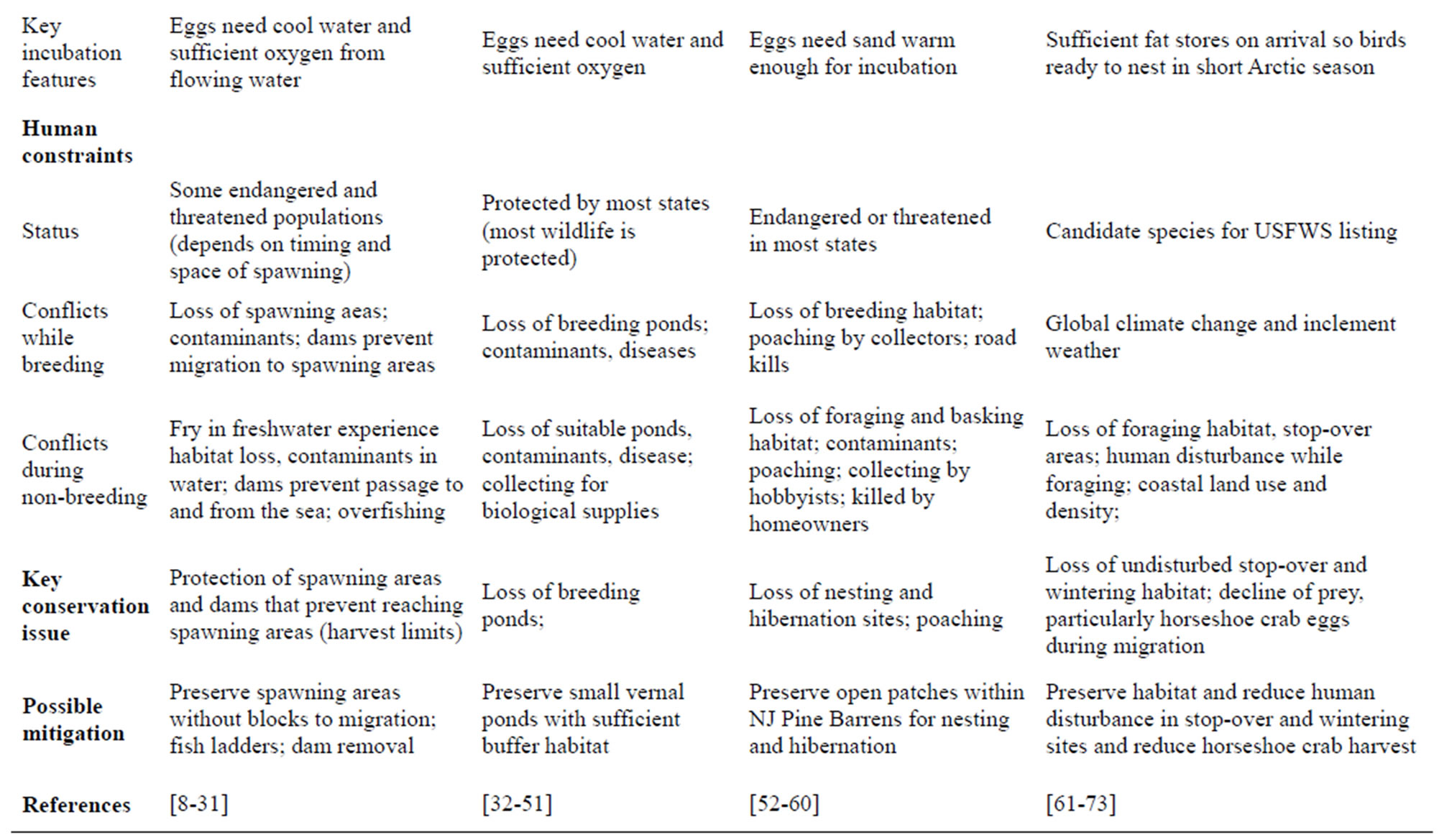
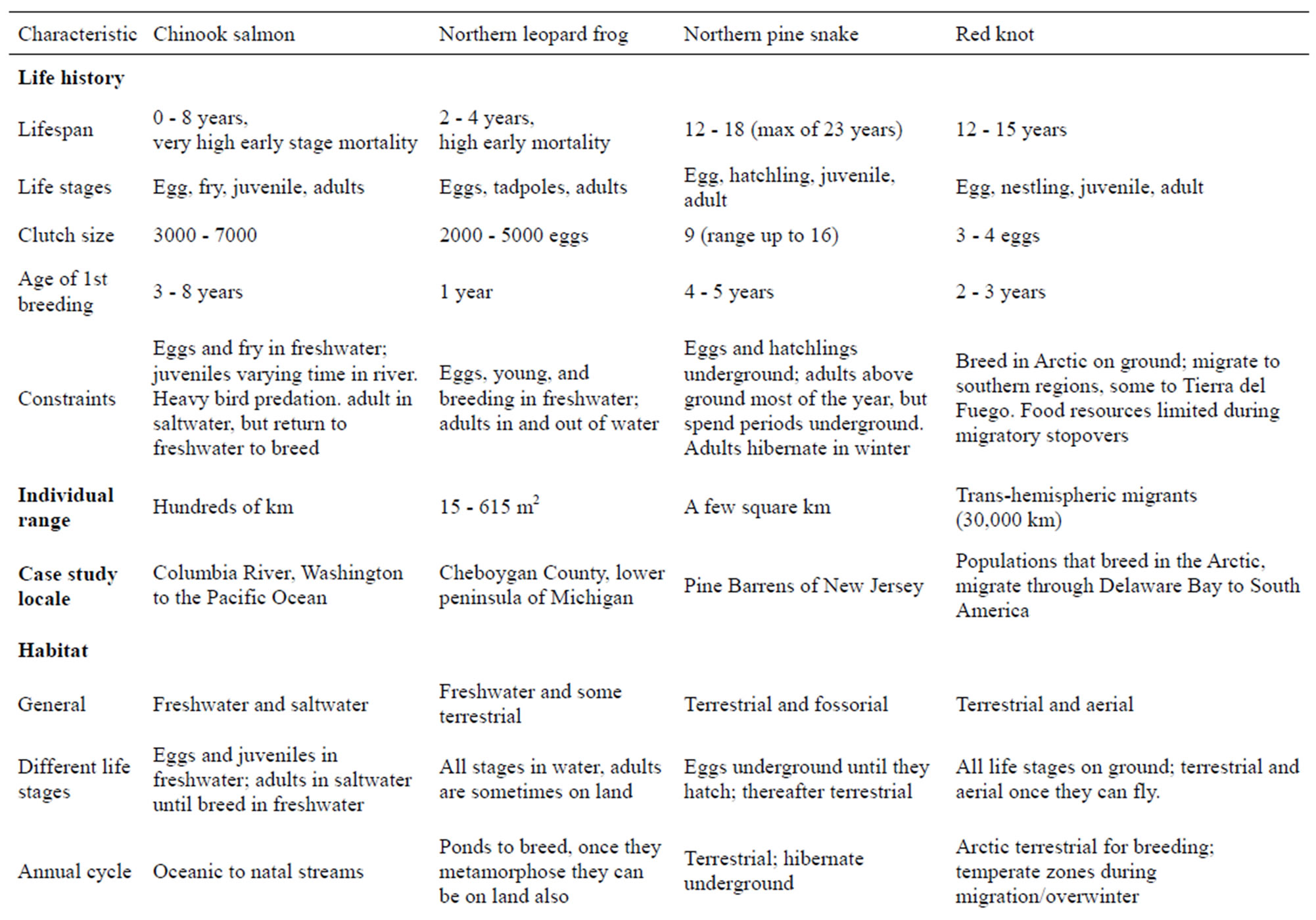
Table 1. Characteristics that result in competing demands among physical features, species requirements, and human constraints. Table is based on the literature (see references below) and our combined field experience.
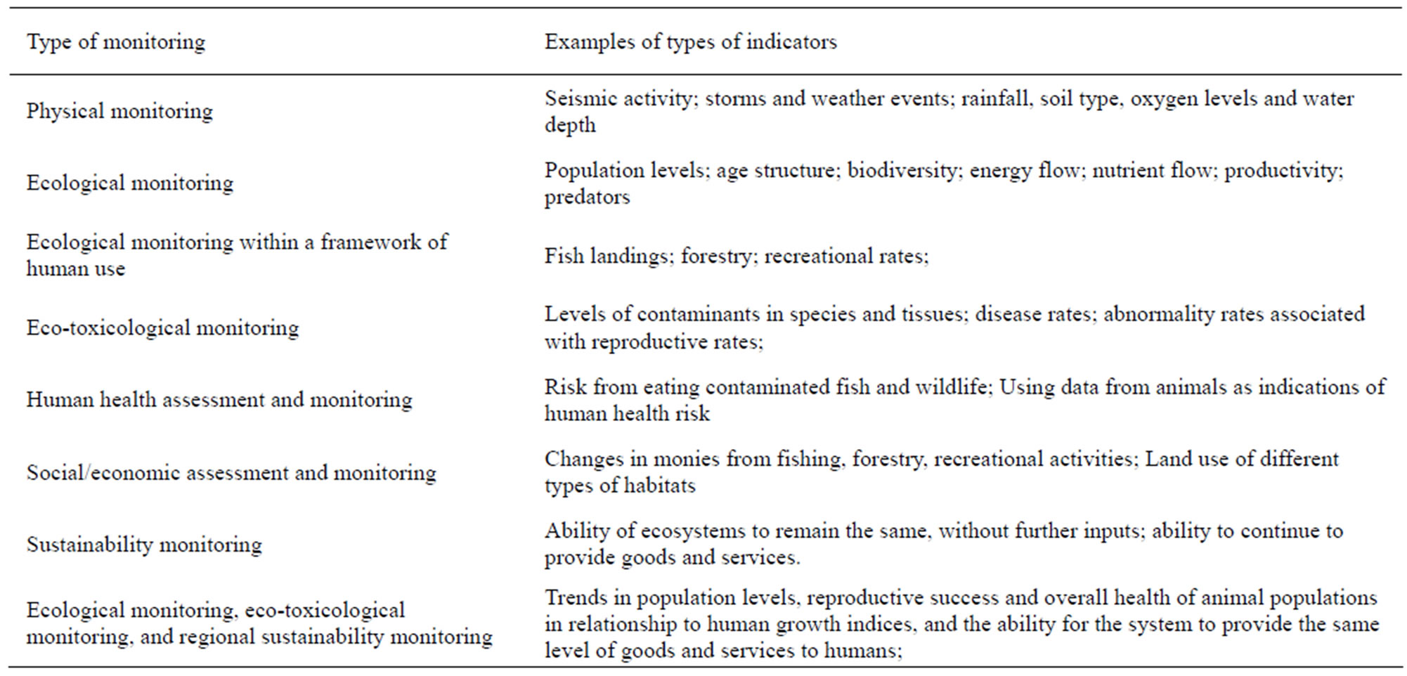
Table 2. Types of monitoring required to adequately assess environmental conditions, with general examples of types of monitoring.
vest limits [13], genetic stability, and the large-scale supplementation of populations with hatchery fish [14]. Harvests of Chinook salmon have been as high as 19.5 million Kg in 1889 from the Columbia River system, but by 1960 it had declined to less than 5 million Kg [15]. Now, sometimes hatchery fish produce more offspring that reach adulthood than wild salmon in the same rivers reproducing naturally [16]. The Columbia River Basin once had the largest salmon runs in the world (10 - 16 million fish), but these have decreased to about a million upriver salmon [9].Chinook run up river spring, summer and fall. The much smaller spring and summer runs are considered endangered [17]. The difficulty is that all (or part) of each run occurs in different tributaries and sections of the main Columbia River. Salmon declines have resulted in cultural deprivation for some Native American tribes that have been using salmon from the Columbia River Basin for about 9000 years [8,18]. Salmon runs on the Columbia River have been severely impacted by dams that prevent access to their traditional upstream spawning areas [19]. Habitat quality has also been affected by altering water level and current characteristics. Thus, the biggest habitat difficulty is the inability of salmon to reach most of their traditional spawning grounds. The Pacific Northwest is embroiled in major public policy debates about how to restore Pacific salmon. In this paper we use Chinook salmon as the bioindicator, and hereafter information pertains to this species. Chinook salmon are the most abundant species of salmon in the Columbia River Basin [9,15].
Salmon eggs are laid and hatch in gravel nests in flowing fresh water. Young spend a variable part of their lives (months to years) in freshwater and thereafter swim to the ocean, where they mature over a period of years (1 - 5 years, [20]). Some Chinook salmon spend their entire lives in freshwater [21]. Adults come back to their natal river to spawn (and die there). When adult salmon come upstream, they excavate nests (in spawning areas called redds) in gravelly sediment. Those that spawn in the river (summer and fall runs) typically spend less than a year in freshwater before migrating to the sea [17], and some reach the ocean within 3 months of emergence [22]. Some salmon are capable of swimming the 2600 river km from Idaho to the Columbia River and back within 4 months [20]. Some males have several strategies; there is a continuum of different strategies [20]. That is, males may mature a year earlier than females from their same cohort (=precocious maturation). Determining the maximum times in each stage and location is difficult. As a further complication, there are two life history strategies that occur in the Columbia River-those that migrate to the ocean in their first year, and those that spend a full year in freshwater [23].
Selection of nest sites within spawning areas (redds) is critical to reproductive success, and spawning habitat is limited by deep water and low water velocity [19]. Important substrate characteristics are pebble count, grain size in the nesting area, water depth, and water velocity. The spawning areas need downward flow of water through the nest where eggs are located (eggs are 20 cm below surface). Fall spawning criteria developed by Hanrahan et al. [19] included water depth (0.30 - 9.5 m), velocity (0.23 - 2.25 m/sec), substrate (25 - 305 mm grain size), and channel bed slope (0 - 5 % slope). The salmon prefer nesting in areas with water velocities greater than 1 m/s, and where streamflow fluctuations are
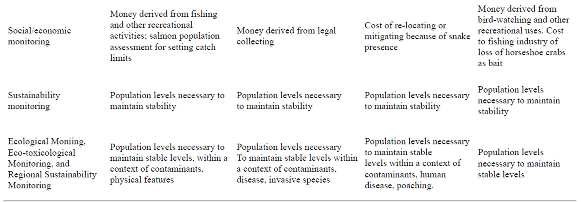
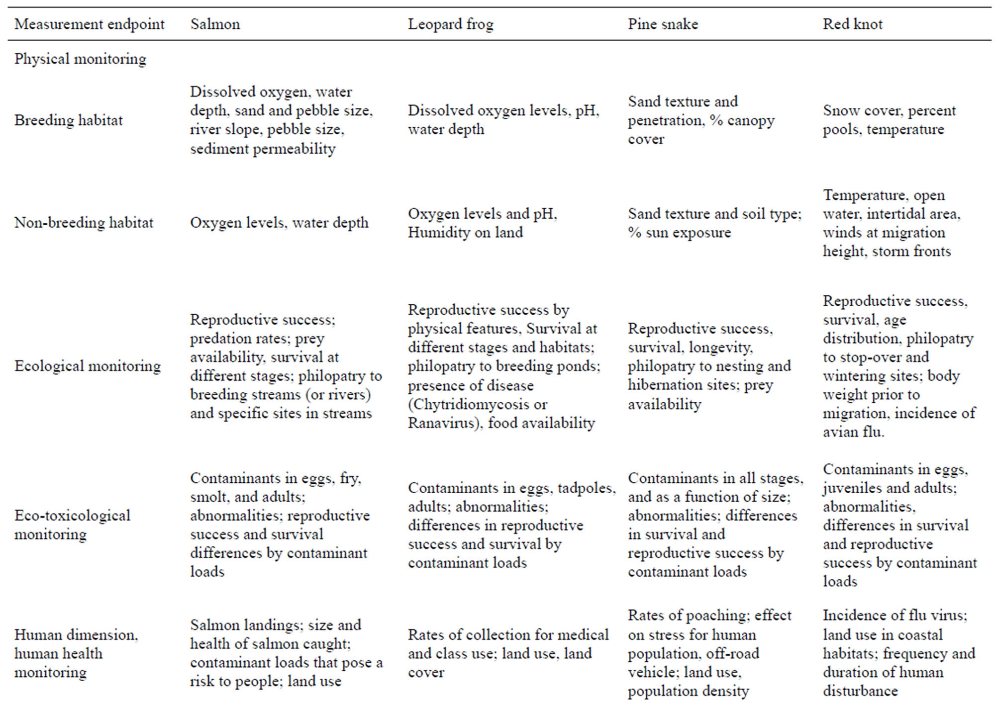
Table 3. Biomarkers or measurement endpoints for habitat assessment. The bioindicators are used to illustrate the breadth of the ecological and habitat data needed to ensure sustainability. Based on literature and our research experience.
reduced [24]. Excessive fine sediment impairs egg survival [25]. Geist et al. [26] estimated that water velocities between 1.4 and 2 m/s, water depth 2 - 4 m, and lateral slope of the riverbed of less than 4% was ideal for spawning habitat. Optimum dissolved oxygen was about 9 mg/L [27]. Thus, there are specific habitat requirements for spawning Chinook salmon, and these are threatened by climate change (reduced stream flow [28]). While most attention has been devoted to habitat characteristics within the freshwater systems, landscape scale habitat parameters are important in predicting recruitment of Chinook salmon [29]. Three factors accounted for salmon recruitment: % of land that was urban, proportion of stream length failing to meeting water quality standards, and index of ability of streams to recover from sediment flow events—perhaps a surrogate for reduced cover and increased siltation [29]. Agricultural runoff also must be considered. Additionally, there is concern about the potential impacts of chromium (hexavalent) on salmon eggs and young [10], although some studies have failed to find an effect on eggs [30]. Further, tern and cormorant predation at the mouth of the Columbia River can be severe (up to 17% of smolt) because of the presence of dense nesting colonies [31].
Assessment endpoints primarily relate to freshwater characteristics, and include water flow, water depth, pebble size, bank slope, and dissolved oxygen (physical monitoring), conspecific nesting density, food availability and reproductive measures (ecological monitoring), contaminants and abnormalities in different stages (ecotoxicological monitoring), salmon landings, size and health of the salmon, contaminant levels toxic for consumption (human health monitoring), and monies derived from salmon fishing licenses, fish hatcheries, and other businesses associated with salmon fishing, as well as the cultural and nutritional benefits for Native American Tribes (cultural/economic monitoring) (Table 3). Trends in salmon numbers and spawning activity (sustainability), is of concern.
3.2. Northern Leopard Frog
Frogs have experienced unprecedented worldwide declines in recent decades, leading to regional extirpations and global extinctions [32]. As a result, frogs, along with the other members of the Amphibia (e.g. salamanders, caecilians) now constitute the most threatened major vertebrate group on earth [33,34]. The leopard frog or Rana pipiens (=Lithobates pipiens) complex is genetically diverse and taxonomically complicated [35], and may represent more species than currently recognized [36]. Leopard frogs were considered historically abundant throughout many parts of their range [37], but declines have been reported from each of the widespread species, including the southern leopard frog (R. sphenocephala) [38] and plains leopard frog (R. blarii) [39]. However, the species that has arguably suffered the greatest impacts is nominate species itself, the northern leopard frog (R. pipiens), which has declined or disappeared entirely from many regions [40]. Northern leopard frogs are now endangered in western Canada and Washington State, and are considered critically imperiled in Montana, New Mexico, Oregon, and Texas. This species is still common in some regions however and is harvested for research, food and bait [41,42].
Northern leopard frogs range from New England and Nova Scotia west to the Pacific coast states and British Columbia. They are restricted to aquatic environments during the egg and larval (tadpole) stages of their life cycle but expand to moist terrestrial environments as frogs. General habitat requirements include cover, moisture, and foraging areas, and adults return to water to hibernate and congregate for breeding assemblages that can include hundreds of breeding individuals in total [43], with males calling to attract females. The frogs can be found in bogs and occasional forest patches, but are most often associated with grassy fields and meadows in close proximity to wetlands [40]. Leopard frogs encounter many predators (including humans) which they avoid by jumping into vegetation or water.
Breeding typically occurs during a narrow period in the spring, after the onset of 10˚C temperatures, and fertilization and egg success decreases with pH values of 6.5 - 5.5 and lower [40]. Thus they prefer to breed in less acidic wetlands that are also no deeper than 1 - 2 m and contain aquatic vegetation [44] for cover and egg mass attachment. Masses may contain up to 5000 eggs [44] and hatch at variable rates depending on temperature, with ranges from two days at 27.6˚C to five days at 18.5˚C and 17 days at 11.4˚C [45]. Tadpoles metamorphose into frogs in 2 - 6 months depending upon location and elevation [40,42]. Larval development is also faster at higher water temperatures [46] which can provide advantages in terms of food acquisition and lowered predation risk. Eggs and tadpoles are vulnerable to predators in the water, including fish, and breeding adults prefer fishless areas or ephemeral (vernal) wetlands that do not support fish [44,47]. Leopard frogs are also vulnerable to pesticides [48,49], heavy metals such as lead and cadmium [50], and the fungal disease chytridiomycosis [51].
The primary habitat requirements are water (egg-laying, tadpoles), suitable water temperatures (development), moisture in terrestrial habitats (adults), open canopied habitats (foraging), and cover in both aquatic (predator avoidance and egg attachment) and terrestrial environments (predator avoidance). In addition, they need water that is free of pesticides and heavy metals. Habitat requirements depend upon life stage.
Assessment endpoints for leopard frogs include: water that is deep enough for development of eggs and tadpoles and to avoid freezing during hibernation, warm temperatures for egg and tadpole development (physical assessment), water that is not so deep and permanent that it can harbor predators, including fish, sufficient connectivity between suitable habitats to ensure genetic viability, available moist terrestrial habitat with cover for adults to forage when they are not breeding (ecological assessment), water and food that is free from pesticides and heavy metals (ecotoxicological monitoring), population stability, contaminant levels, and developmental abnormalities that can allow frogs to serve as sentinels of environmental contamination, and to be safely consumed (human health assessment), and lack of overexploitation by the medical industry and classroom dissections (economic monitoring). These measures can be combined to provide an overall integration of the different levels of assessment.
3.3. Northern Pine Snake
Northern pine snakes reach the northern limit of their range in southern New Jersey, and are found in disjunct populations in Kentucky, Tennessee, Virginia, North Carolina, South Carolina and Georgia. In New Jersey and other states the species is endangered, threatened, or species of special concern [52]. The main threat faced by pine snakes throughout their range is habitat loss [53,54], although predation, mortality due to road and off-road vehicles, and poaching of eggs, hatchlings and adults are conservation concerns. The presence of off-road vehicles results in a decrease of recruitment of hatchlings from 28 % to about 15 %; thus presence of off road vehicles can cut recruitment nearly in half [55].
In New Jersey, the stronghold of their distribution, nesting female pine snakes excavate long tunnels in bare sand, and lay their eggs in a chamber at the end of the tunnel. Full sun penetration to the ground is necessary to allow for successful incubation, and to provide sufficient heat that fledglings are not behaviorally impaired upon hatching (Temperatures over 24˚C, [56]. Females show high site fidelity to nest sites, and such site-specific habitats need to be protected [57]. Similarly, pine snakes require fairly open patches for hibernation sites to keep the soil from freezing, while still allowing the snakes to be above the gravel layer that impedes digging [58,59]. Most snakes hibernate at depths of 50 - 111 cm (maximum of 200 cm), indicating that sand depths without gravel need to be at least 111 cm to avoid winter temperature stresses [58]. Pine snakes also show fidelity to hibernation sites, and optimal sites are occupied continuously for over 20 years [54], suggesting that these specific habitat sites need to be protected.
Pine Snakes occupy mixed oak-pine forest which provides habitat for basking, resting, and foraging; in New Jersey they spend only about 5% of their time in lowland pine forests, and are mainly in upland pine-oak forests with open areas for nesting, basking, and hibernating [60]. Radio-tracked snakes spend about 40% of their time in old abandoned railroad beds, farm houses, farmlands, and areas burned for deer production [60]. Gerald et al. [52] similarly found that northern pine snakes in Tennessee primarily used disturbed habitats. Paved roads are barriers to movement, mating, genetic transfer among populations [53]. Mortality from highway traffic and offroad vehicles reduce nesting success and recruitment to nearly zero [55]. Pine Snakes are sedentary, and their home range in New Jersey averages about 70 ha, with a maximum of nearly 190 ha [60]. Although individual snakes require limited habitat, large undisturbed tracts of suitable habitat are necessary to maintain viable populations [53].
The habitat features that require assessment (Table 1) include suitability of sand for digging, stability of the sand so that nests do not collapse on the eggs, for full sun penetration that provides sufficient heat for incubation and hibernation, and intermixed pine forest, open areas and old fields for hunting prey [53,54]. Measurement endpoints include sand texture and sand penetration (physical monitoring), other conspecifics for mating, reproductive success, survival, and longevity (ecological), contaminant levels (ecotoxicology), poaching rates, road kill rates, and mortality and habitat destruction by offroad vehicles (human dimensions), and cost of re-locating snakes displaced by development (social/economic, Table 3). This monitoring is particularly critical because their near range-wide threatened or endangered status means that developers are required to consider pine snake populations in development plans.
3.4. Red Knot
Red knots are medium-size shorebirds (100 - 200 g) that breed in the Arctic and make long-distance migrations of up to 30,000 km to the southern hemisphere [61]. The eastern North American subspecies (Calidris c. rufa), winters along the Atlantic coast as far south as Tierra del Fuego [62]. Any individual Knot encounters a range of natural and human altered habitats. The species has declined drastically in the past 30 years. Current estimates show that only 30,000 Knots remain in the Western Hemisphere [63]. The Tierra del Fuego segment of the Knot (Calidris. c. rufa) population may have declined more than other populations [62,64], suggesting the importance of developing habitat measurement endpoints for wintering grounds.
Knots feed on tiny invertebrates along the tideline or in mudflats [65]. In spring, northbound migrants arrive in Delaware Bay for a two-three-week stopover. Their dependence on the eggs of horseshoe crabs (Limulus polyphemus) during this stopover is well known, largely because overharvesting of horseshoe crabs by fishermen has decreased the availability of the eggs for shorebirds. A significant proportion of the northbound migrants stop in Delaware Bay [66]. During their brief stopover, the knots need to nearly double their weight to allow for the long migration north to the Arctic, and to have sufficient fat resources to lay eggs [61,67]. They arrive on the wet Arctic tundra just after snow melt, when food is still scarce, and females deplete their body fat to lay their eggs.
The species has both short-distance migrants, and long-distance migrants, which results in very different habitat requirements. Of the four bioindicator species discussed in this paper, red knots have the longest distance migration, accounting for much of their risk [62, 68]. Because red knots depend upon coastal and estuarine environments during most of their life cycle, global warming and increased sea level will result in severe habitat loss. Galbraith et al. [69] predicted that major intertidal habitat losses for shorebirds in bays in Washington, California, Texas, and New Jersey/Delaware will range from 20 to 70 %.
The habitat features that require assessment (Table 1) include snow-free nesting areas with nearby water for foraging, tidal beaches and mudflats for foraging at stopover and migration sites, sufficient and available prey during the winter, presence of spawning horseshoe crabs, and sufficient roosting sites safe from predators and human disturbance during their migration and wintering stages [70]. Measurement endpoints include: % snow cover and % available foraging pools in the Arctic, Arctic temperatures, amount of available tidal flats for feeding (physical monitoring), number of horseshoe crab eggs, density of prey (invertebrates), reproductive success, survival, longevity, populations levels at particular stopover or wintering sites (ecological monitoring), contaminant levels in eggs, feathers and other tissues (ecotoxicology), % habitat without human disturbance and % flu virus on migration (they carry avian influenza [71], human health), and % loss of fishing and recreational activities due to beach closures during migration (economic) (Table 3). The aim of assessment is to maintain healthy populations of both short-distance and long-distance migrants. Since habitats in the two regions differ, different measurement endpoints may be required. For example, endpoints for short-distance migrants may relate to amount of available tidal exposure, and to human disturbance [72, 73]. In contrast, measurement endpoints for long-distance migrants that fly to Tierra del Fuego may include body weight prior to migration, winds at migration height, fog, and storm fronts on migration route, limited intertidal space, human harvesting for food, and prey abundance.
4. DISCUSSION
4.1. Natural History and Life Cycle Considerations
The species selected as bioindicator have different individual ranges (sedentary to trans-equatorial migrations), different types of habitats (freshwater vs saltwater), and live in different media (water, land, air). They have different life-spans, from a very few years for leopard frog, to 5 to 8 years for salmon, to 20 to 30 years for pine snakes and red knots. Frogs and salmon undergo several metamorphic stages. Birds and snakes lay eggs that hatch into juveniles which take two to four years to mature. Additionally, their existence is threatened by different degrees of human activities. Salmon are important recreational, commercial, and cultural fish (especially for Native Americans), while human interest in the others is for species survival and the degree of conflict between their survival and the activities of people (e.g. development). Some frogs, however, are also consumed, making them of interest commercially, recreationally, and in terms of contaminant loads.
Habitat complexity is another continuum that affects population stability and sustainability. In general, habitat complexity varies as a function of geographical range. And here, geographical range must be considered in terms of individual versus species ranges. Because frogs and snakes are sedentary, with relatively small home ranges, the complexity of the measurement endpoints needed to assess habitat suitability are more limited than for species with larger ranges, more habitat complexity, and that use more ecosystem components (e.g. water, land, air; birds). However, since the overall species range of frogs and pine snakes may include larger geographical ranges, habitat availability with the larger species geographical range must also be considered.
Species that move between different media, or different components within media types, have more complex habitat requirements than those that do not. For example, salmon move between freshwater and salt water, frogs move between freshwater and land, and birds move between land and the air. In contrast, pine snakes move only between the land surface and below (to dig nests or to hibernate). Each habitat or media type has different constraints.
4.2. Critical Habitat
One of the key features that emerged from our examination of these four bioindicators is the importance of critical habitat, in specific locations, for the species which are endangered, threatened, or species of special concern (all except northern leopard frog). For example, a large percentage of the Chinook salmon in the Columbia River spawn along the Hanford Reach [10], pine snakes use the same nest sites and hibernacula for many years [54], and red knots migrate through Delaware Bay and other stopover sites year after year [62]. Thus it is these critical habitats that require the development of biomarkers or measurement endpoints that can be used to: 1) assess current habitat; 2) set remediation or restoration habitat goals; 3) evaluate the efficacy of conservation, remediation or restoration projects; and 4) protect habitat for long-term population stability and sustainability. The specific endpoints listed in Table 3 are those that can be used to address the aforementioned objectives.
Critical habitats, such as the Hanford Reach for salmon or specific nesting/hibernation places for pine snakes, are specific places geographically. And in most cases, these places need to be evaluated and protected. However, it is particular features of these habitats that make them critical, whether it is water depth, water velocity and substrate) size for developing eggs of salmon, or sand penetration, sand stability, and temperature for developing eggs of pine snakes. The specific features that are essential to identify and measure are those that lead to improved development and hatching of eggs, continued growth and development of young (regardless of whether they are called fry or juveniles, and continued growth, foraging, and migratory behavior of juveniles and adults.
Northern leopard frog was selected as a bioindicator specifically because, unlike the other three species, they are widespread geographically, and generally not threatened, although overall declining trends are apparent across their range. Instead they are rather common and widespread. Even so, they have specific habitat requirements that require assessment, and some of the measurement endpoints (e.g. water temperature, water oxygen levels, vegetative cover) are the same as those required by the other bioindicators. It is not the biomarkers or measurement endpoints that differ, just that the available, suitable habitat is more widespread, and thus not as “critical” as for the other species. The other three species indicate clearly that suitable habitat is limited, that it is imperative to identify the habitat parameters that are relevant to assess, and that it is essential to quantify the range of endpoint values that are necessary to maintain or increase reproductive rates that can sustain stable populations.
It is increasingly clear that sustaining stable populations of species within a context of habitat assessment, restoration, protection, and long-term stewardship require models. Habitat models can be used to design and implement protection, remediation and restoration, to evaluate habitat sustainability of existing populations, to evaluate the effectiveness of remediation, to select among restoration alternatives, and to predict the long-term sustainability of populations.
Salmon are the species that have been subjected to the most modeling because of their economic, recreational, and cultural significance. Salmon have been part of tribal culture for over 9000 years [74]. Many of the models for salmon have been developed to examine stock recruitment, escapement rates, and fish takes [75], hydrology [76], habitat characteristics [26], and survivorship [25]. The Honea et al. [25] model indicated that population status could be improved by streambed restoration, with the reduction in the percentage of fine sediments. Models that combine the biological and physical factors affecting population stability will increase our understanding of options for restoration and management of viable Chinook salmon populations in the Columbia River and elsewhere. Further, dynamic rather than static models are required to accurately predict spawning activity (e.g. streamflow fluctuations over redds.
Little modeling has been conducted for habitat needs for frogs, for understanding the factors leading to Worldwide declines in amphibians, or for understanding why leopard frogs have disappeared from some areas. Modeling for pine snakes has related to viable population sizes, and to habitat and landscape scale features necessary to maintain a viable population [53]. Modeling of habitat requirements for shorebirds has mainly involved understanding the effect of different human disturbance regimes on foraging shorebirds [73], and predicting the effect of global change and sea level rise on available intertidal habitat for foraging and roosting shorebirds [69]. Human disturbance models have been used to evaluate the suitability of foraging habitat as a function of the number of disturbances, with the aim of managing coastal habitats during critical migration and stopover times of shorebirds [75]. Thus, there is a wide range of models that have been applied to the different bioindicator species, and understanding habitat requirements for management purposes for most species would benefit from the application of all the models.
4.3. Conclusions: Measurement Endpoints and Biomarkers
Selecting endpoints for assessment and monitoring is critical for managers, public policy-makers (who partly control funding and resource allocation), and the public, as well as for people engaged in remediation and restoration of habitat. Measurement endpoints should be quantifiable, easy to measure, be measured by easily-trained personnel, reflect environmental change that is meaningful, cost-effective, of interest to the public, and easy to interpret by scientists, managers, public policy makers, and the public [77-79].
The key to sustaining viable populations is monitoring of species numbers, reproductive success, and abnormalities caused by environmental stressors. But equally important is monitoring the physical and biological characteristics of habitat necessary to sustain populations. The bioindicators discussed in this paper were selected to reflect a range of habitat types, and illustrate biomarkers or measurement endpoints that can be used to evaluate habitat. It is clear from these examples that refinements in endpoints depend upon the level of knowledge about species habitat needs. Thus, for salmon, where there are many papers that deal with very specific habitat requirements of spawning salmon in different parts of the Columbia River, the measurement endpoints to apply to this, or other rivers, are more clearly defined. Further, since specific requirements for gravel size, water depth, and water velocity have been delineated, these can be compared to these physical parameters in salmon spawning elsewhere.
In contrast, there are far fewer studies of specific nesting habitat requirements for leopard frogs and pine snakes, and even fewer for red knot, since they nest in the Arctic where environmental conditions make study difficult and where habitat shifts in the species complicate location. Attention has been devoted, however, to determining the habitat features essential to foraging during stopovers areas for red knot, mainly because habitat is most limiting during these times, they stopover in temperate regions, where global warming is expected to have severe effects [69].
The bioindicators discussed in this paper illustrate the importance of using a diverse array of assessment methods (physical, ecological, ecotoxicology, human health/ dimensions, sustainability) to evaluate habitat requirements of individual species and groups of species. This information could then be used for habitat management, remediation and restoration, and long-term sustainability planning to integrate human and ecological needs. Without evaluation at all levels of assessment, long-term sustainability of monitoring programs necessary to inform habitat management for species will not engage the public enough to sustain long term funding and support.
5. ACKNOWLEDGEMENTS
We thank the many people who we have discussed these topics with us, or who have helped in the research, including L. Bliss, A. Dey, E. DeVito, C. Duncan, C. Frank, M. Gilbertson, C. Jeitner, D. Jenkins, C. Minton, T. Pittfield, H. Sitters, and other field volunteers. We thank the many organizations and individuals who contributed throughout this research. This project was mainly funded by the Consortium for Risk Evaluation with Stakeholder Participation (Department of Energy, DE-FC01-86EW07053), with additional funding from NIEHS ((P30ES 005022), U.S. Fish and Wildlife Foundation, NJ Department of Environmental Protection (Endangered and Nongame Program), Conserve Wildlife Foundation of New Jersey, Endangered and Nongame Species Program of the NJ Department of Environmental Protection, and Rutgers University.The views and opinions expressed in this paper are those of the authors, and do not represent the funding agencies.
REFERENCES
- National Research Council (2008) Public participation in environmental assessment and decision making. National Academy Press, Washington DC.
- European Environment Agency (2003) Environmental indicators: Typology and use in reporting. EEA, Copenhagen.
- National Oceanic and Atmospheric Administration (2011) The Gulf of Mexico at a Glance. NOAA, Department of Commerce, Washington DC.
- Environmental Protection Agency (2009) Environmental justice: Compliance and environment. http://www.epa.gov/environmentaljustice
- Burger, J. (2011) Stakeholders and scientists: Achieving implementable solutions to energy and environmental issues. Springer, New York. doi:10.1007/978-1-4419-8813-3
- FWS (United States Fish & Wildlife Service) (2012) Species profile: Chinook salmon. http://ecos.fws.gov/speciesProfile/profile/speciesProfile.action?spcode=E06D
- Narum, S.R., Hess, J.E. and Metala, A.P. (2010) Examining genetic lineages of Chinook Salmon in the Colombia River Basin. Transactions of the American Fisheries Society, 139, 1465-1477. doi:10.1577/T09-150.1
- Columbia River Inter-Tribal Fish Commission (2013) We are Salmon people. http://critfc.org/salmon-culture/columbia-river-salmon/columbia-river-salmon-species
- Environmental Protection Agency (2009) Columbia River Basin: State of the River Report for Toxics. EPA 910- R-08-004.
- Oregon Hanford Waste Board (2002) River without waste: Recommendations for Protecting the Columbia River from Hanford Site Nuclear Waste. USDOE, Hanford.
- Dauble, D.D. and Watson, D.G. (1997) Status of fall Chinook salmon populations in the mid-Columbia River, 1948-1992. North American Journal of Fisheries Management, 17, 283-300. doi:10.1577/1548-8675(1997)017<0283:SOFCSP>2.3.CO;2
- Dauble, D.D., Hanrahan, T.P., Geist, D.R. and Parsley, M.J. (2003) Impacts of the Columbia River hydroelectric system on main-stem habitats of fall Chinook salmon. North American Journal of Fisheries Management, 23, 641-659. doi:10.1577/M02-013
- Hyun, S.-Y., Keefer, M.W., Fryer, J.D., Jepson, M.A., Sharma, R., Caudill, C.C., Whiteaker, J.M. and Naughton, G.P. (2012) Population-specific escapement of Columbia River fall Chinook salmon: Tradeoffs among estimation techniques. Fisheries Research, Vol. 129-130, pp. 82-93. doi:10.1016/j.fishres.2012.06.013
- Kostow, K. (2012) Strategies for reducing the ecological risks of hatchery programs: Case studies from the Pacific Northwest. Environmental Biology of Fishes, 94, 285-310. doi:10.1007/s10641-011-9868-1
- Fulton, L.A. (1968) Spawning areas and abundance of Chinook salmon (Oncorhynchus tshawytscha) in the Columbia River Basin—Past and present. US Fish and Wildlife Service, Special Scientific Report, Fisheries No. 571, Washington DC.
- Hess, M.A., Rabe, G.D., Vogel, J.L., Stephenson, J.J., Nelson, D.D. and Narum, S.R. (2012) Supportive breeding boosts natural population abundance with minimal negative impacts on fitness of a wild population of Chinook salmon. Molecular Ecology, 21, 5236-5250. doi:10.1111/mec.12046
- Chelan (Chelan County Public Utility) (2012) Mid-Columbia Salmon species. http://www.chelanpud.org/mid-columbia-salmon-species.html
- Landeen, D. and Pinkham, A. (1999) Salmon and his people. Quaternary Research, 62, 1-8.
- Hanrahan, T.P., Dauble, D.D. and Geist, D.R. (2004) An estimate of Chinook salmon (Oncorhynchus tshawytscha) spawning habitat and red capacity upstream of a migration barrier in the upper Columbia River. Canadian Journal of Fisheries and Aquaculture Science, 61, 23-33. doi:10.1139/f03-140
- Johnson, J., Johnson, T. and Copeland, T. (2012) Defining life histories of precocious male parr, minijack, and jack Chinook Salmon using scale patterns. Transactions of the American Fisheries Society, 141, 1545-1556. doi:10.1080/00028487.2012.705256
- Connor, W. P., Sneva, J.G., Tiffan, K.E., Steinhorst, R.K. and Ross, D. (2005) Two alternative juvenile life history types for fall Chinook salmon in the Snake River Basin. Transactions of the American Fisheries Society, 134, 291- 305. doi:10.1577/T03-131.1
- Dauble, D.D. and Geist, D.R. (2000) Comparison of mainstem spawning habitats for two populations of fall Chinook salmon in the Columbia River Basin. Regulated Rivers: Research & Management, 16, 345-361. doi:10.1002/1099-1646(200007/08)16:4<345::AID-RRR577>3.0.CO;2-R
- Sharma, R. and Quinn, T.P. (2012) Linkages between the life history type and migration pathways in freshwater and marine environments for Chinook salmon, Oncorhynchus tshawytscha. Acta Oecologica, 41, 1-13. doi:10.1016/j.actao.2012.03.002
- Hatten, J.R., Tiffan, K.F., Anglin, D.R., Haeseker, S.L., Skalicky, J.J. and Schaller, H. (2009) A spatial model to assess the effects of hydropower operations on Columbia River fall Chinook salmon spawning habitat. North American Journal of Fisheries Management, 29, 1379-1405. doi:10.1577/M08-053.1
- Honea, J.M., Jorgensen, J.C., McClure, M.M., Cooney, T.D., Engie, K., Holzer, D.M. and Hilborn, R. (2009) Evaluating habitat effects on population status: Influence of habitat restoration on spring-run Chinook salmon. Freshwater Biology, 54, 1576-1592. doi:10.1111/j.1365-2427.2009.02208.x
- Geist, D.R., Jones, J., Murray, C.J. and Dauble, D.D. (2000) Suitability criteria analyzed at the spatial scale of redd clusters improved estimates of fall Chinook salmon (Oncorhynchus tshawytscha) spawning habitat use in the Hanford Reach, Columbia River. Canadian Journal of Fisheries and Aquatic Sciences, 57, 1636-1646. doi:10.1139/f00-101
- Geist, D.R. (2000) Hyporhelc discharge of river water into fall Chinook salmon spawning areas in the Hanford Reach, Columbia River. Canadian Journal of Fisheries and Aquatic Sciences, 57, 1647-1656. doi:10.1139/f00-102
- Donley, E.E., Naiman, R.J. and Marineau, M.D. (2012) Strategic planning for instream flow restoration: A case study of potential climate change impacts in the central Columbia River basin. Global Change Biology, 18, 3071- 3086. doi:10.1111/j.1365-2486.2012.02773.x
- Regetz, J. (2003) Landscale-level constraints on recruitment of Chinook salmon (Oncorhynchus tshawytscha) in the Columbia River, USA. Aquatic Conservation: Marine and Freshwater Ecosystems, 13, 35-49. doi:10.1002/aqc.524
- Farag, A.M., Harper, D.D., Cleveland, L., Brumbaugh, W.G. and Little, E.E. (2006) The potential for chromium to affect the fertilization process of Chinook salmon (Oncorhynchus tshawytscha) in the Hanford Reach of the Columbia River, Washington, USA. Archives of Environmental Contamination and Toxicology, 50, 575-579. doi:10.1007/s00244-005-0010-2
- Good, T., McClure, M.M., Sandford, B.P., Barnas, K.A., Marsh, D.M., Ryan, B.A. and Casillas, E. (2007) Quantifying the effect of the Caspian tern predation on threatened and endangered Pacific salmon in the Columbia River estuary. Endangered Species Research, 3, 11-21. doi:10.3354/esr003011
- Stuart, S.C., Chanson, J.S., Cox, N.A., Young, B.E., Rodrigues, A.S.L., Fishman, D.L. and Waller, R.W. (2004) Status and trends of amphibian declines and extinctions. Science, 306, 1783. doi:10.1126/science.1103538
- Ballie, J.E.M., Hilton-Tarylor, C. and Stuart, S.N. (2004) IUCN red list of threatened species: A global species assessment. IUCN Publications Services Unit, Cambridge. doi:10.2305/IUCN.CH.2005.3.en
- Blaustein, A.R., Wake, D.B. and Sousa, W.P. (1994) Amphibian declines: Judging stability, persistence, and susceptibility of populations to local and global extinctions. Conservation Biology, 8, 60-71. doi:10.1046/j.1523-1739.1994.08010060.x
- Hillis, D.M. (1988) Systematics of the Rana pipiens complex: Puzzle and paradigm. Annual review of Ecology and Systematics, 19, 39-63. doi:10.1146/annurev.es.19.110188.000351
- Newman, C.E., Feinberg, J.A., Rissler, L.J., Burger, J. and Shaffer, H.B. (2012) A new species of leopard frog (Anura:Ranidae) from the urban northeastern US. Molecular Phylogenetics and Evolution, 63, 445-455.
- Lannoo, M. (2005) Amphibian declines: The conservation status of United States species. University of California Press, Berkeley.
- Daszak, P., Scott, D.E., Kilpatrick, A.M., Faggioni, C., Gibbons, J.W. and Porter, D. (2005) Amphibian population declines at Savannah River Site are linked to climate not chytridiomycosis. Ecology, 86, 3232-3237. doi:10.1890/05-0598
- Clarkson, R.W. and Rorabaugh, J.C. (1989) Status of leopard frogs (Rana pipiens complex) in Arizona and southeastern California. Southwestern Naturalist, 34, 531-538. doi:10.2307/3671513
- Rorabaugh, J.C. (2005) Rana pipiens schreber, 1782, northern leopard frog. In: Lannoo, M., Ed., Amphibian Declines: The Conservation Status of United States Species, University of California Press, Berkeley, 570-577.
- Woodhams, D.C., Hyatt, A.D., Boyle, D.G. and RollinsSmith, L.A. (2008) The northern leopard frog Rana pipiens is a widespread reservoir species harboring Batrachochytrium dendrobatidis in North America. Herpetological Review, 39, 66-68.
- Wagner, G. (1997) Status of the northern leopard frog (Rana pipiens) in Alberta. Wildlife Status Report, No. 9, Alberta Environmental Protection, Edmonton.
- Hoffman, E.A., Schueler, F.W. and Blouin, M.S. (2004) Effective population sizes and temporal stability of genetic structure in Rana pipiens, the northern leopard frog. Evolution, 58, 2536-2545.
- Merrell, D.J. (1968) A comparison of the estimated size and the “effective size” of breeding populations of the leopard frog, Rana pipiens. Evolution, 22, 274-283. doi:10.2307/2406526
- Moore, J.A. (1949) Geographic variation of adaptive characters in Rana pipiens. Evolution, 3, 1-24. doi:10.2307/2405448
- Ultsch, G.R., Bradford, D.F. and Freda, J. (1999) Physiology: Coping with the environment. In: McDiarmid, R.W. and Altig, R., Eds., Tadpoles: The Biology of Anuran Larvae, University of Chicago Press, Berkeley, 189- 214.
- Hecnar, S.J. and M’Closkey, R.T. (1997) The effects of predatory fish on amphibian species richness and distribution. Biological Conservation, 79, 123-131. doi:10.1016/S0006-3207(96)00113-9
- Relyea, R.A. (2004) Synergistic impacts of malathion and predatory stress on six species of North American tadpoles. Environmental Toxicology and Chemistry, 23, 1080- 1084. doi:10.1897/03-259
- Relyea, R.A. (2009) A cocktail of contaminants: How mixtures of pesticides at low concentrations affect aquatic communities. Oecologia, 159, 363-376. doi:10.1007/s00442-008-1213-9
- Gross, J.A., Chen, T.-H. and Karasov, W.H. (2007) Lethal and sublethal effects of chronic cadmium exposure on northern leopard frog (Rana pipiens) tadpoles. Environmental Toxicology and Chemistry, 26, 1192-1197. doi:10.1897/06-479R.1
- Daszak, P., Berger, L., Cunningham, A.A., Hyatt, A.D., Green, D.E. and Speare, R. (1999) Emerging infectious diseases and amphibian population declines. Emerging Infectious Diseases, 5, 735-748. doi:10.3201/eid0506.990601
- Gerald, G.W., Bailey, M.A. and Holmes, N.J. (2006) Habitat utilization of pituophis melanoleucus on Arnold Air Force Base in middle Tennessee. Southwestern Naturalist, 5, 253-264. doi:10.1656/1528-7092(2006)5[253:HUOPMM]2.0.CO;2
- Golden, D.M., Winkler, P., Woerner, P., Fowles, G., Pitts, W. and Jenkins, D. (2009) Status assessment of the Northern Pine Snake (Pituophis m melanoleucus) in New Jersey: An evaluation of trends and threats. New Jersey Department of Environmental Protection, Trenton. http://www.state.nj.us/dep/fgw/ensp/pdf/pine_snake_assessment09.pdf
- Burger, J. and Zappalorti, R.T. (2011) The northern pine snake (Pituophis melanoleucus): Its life history, behavior, and conservation. Nova Science, New York.
- Burger, J., Zappalorit, R.T., Gochfeld, M. and DeVito, E. (2007) Effects of off-road vehicles on reproductive success of pine snakes (Pituophus melanoleucus) in the New Jersey pinelands. Urban Ecosystems, 10, 275-284. doi:10.1007/s11252-007-0022-y
- Burger, J. (1998) Effects of incubation temperature on behavior of hatchling pine snakes: Implications for survival. Behavioral Ecology and Sociobiology, 43, 11-18. doi:10.1007/s002650050461
- Burger, J. and Zappalorti, R.T. (1992) Philopatry and nesting phenology of pine snakes Pituophis melanoleucus in the New Jersey Pine Barrens. Behavioral Ecology and Sociobiology, 30, 331-326. doi:10.1007/BF00170599
- Burger, J., Zappalorti, R.T., Gochfeld, M., Boarman, W.I., Caffrey, M., Doig, M., Garber, S.D., Lauro, B., Mikovsky, M., Safina, C. and Saliva, J. (1988) Hiber-nacula and summer den sites of pine snakes (Pituophis melanoleucus) in the New Jersey Pine Barrens. Journal of Herpetology, 22, 425-433. doi:10.2307/1564337
- Burger, J., Zappalorti, R.T., Dowdell, J., Georgiadis, T., Hill, J. and Gochfeld, M. (1992) Subterranean predation on pine snakes (Pituophis melanoleucus). Journal of Herpetology, 26, 259-263. doi:10.2307/1564879
- Burger, J. and Zappalorti, R.T. (1989) Habitat use by pine snakes (Pituophis melanoleucus) in the New Jersey Pine Barrens: Individual and sexual variation. Journal of Herpetology, 23, 68-73. doi:10.2307/1564318
- Baker, A.J., Gonzalez, P.M., Piersma, T., Niles, L.J., de Lima Serrano do Nascimento, I., Atkinson, P.W., Clark, N.A., Minton, C.D.T., Peck, M.K. and Aarts, G. (2004) Rapid population decline in red knots: Fitness consequences of decreased refuelling rates and late arrival in Delaware Bay. Proceedings of the Royal Society of London, Series B, 271, 875-882. doi:10.1098/rspb.2003.2663
- Niles, L.J., Sitters, H.P., Dey, A.D., Atkinson, P.W., Baker, A.J., Bennett, K.A., Carmona, R., Clark, K.E., Clark, N.A., Espoz, C., González, P.M., Harrington, B.A., Hernández, D.E., Kalasz, K.S., Lathrop, R.G., Matus, R.N., Minton, C.D.T., Morrison, R.I.G., Peck, M.K., Pitts, W., Robinson, R.A. and Serrano, I.L. (2008) Status of the red knot (Calidris canutus rufa) in the western hemisphere. Studies in Avian Biology, 36, 185 p.
- Morrison, R.I.G., Ross, R.K. and Niles, L.J. (2004) Decline sin wintering populations of red knots in southern South America. The Condor, 106, 60-76. doi:10.1650/7372
- Niles, L., Burger, J., Porter, R.R., Dey, A.D., Minton, C.D.T., Gonzalez, P.M., Baker, A.J., Fox, J.W. and Gordon, C. (2010) First results using light level geolocators to track red knots in the western hemisphere show rapid and long intercontinental flights and new details of migration paths. Wader Study Group Bulletin, 117, 1-8.
- Withers, K. (2002) Shorebird use of coastal wetlands and barrier island habitat in the Gulf of Mexico. Science World Journal, 2, 514-536. doi:10.1100/tsw.2002.112
- Niles, L.J., Bart, J., Sitters, H.P., Dey, A.D., Clark, K.E., Atkinson, P.W., Baker, A.J., Bennet, K.A., Kalasz, K.S., Clark, N.A., Clark, N.A., Clark, J., Gillings, S., Gates, A.S., Gonzalez, P.M., Hernandez, D.E., Minton, C.T., Morrison, R.I., Porter, R.R., Ross, R.K. and Veitch, C.R. (2009) Effects of horseshoe crab harvest in delaware bay on red knots: Are harvest restrictions working? Bioscience, 59, 153-164. doi:10.1525/bio.2009.59.2.8
- Morrison, R.I.G., Davidson, N.C. and Wilson, J.R. (2007) Survival of the fattest: Body stores on migration and survival in red knots, Calidris canutus islandica. Journal of Avian Biology, 38, 479-487.
- Burger, J., Gordon, C., Niles, L.J., Newman, J., Forcey, G. and Vlietstra, L. (2011) Risk evaluation for federally listed (roseate tern, piping plover) or candidate (red knot) bird species of in offshore waters: A first step for managing the potential impacts of wind facility development on the Atlantic Outer Continental Shelf. Renewable Energy, 36, 338-351. doi:10.1016/j.renene.2010.06.048
- Galbraith, H, Jones, R., Park, R., Clough, J, HerrodJulius, S., Harrington, B. and Page, G. (2002) Global climate change and sea level rise: Potential losses of intertidal habitat for shorebirds. Waterbirds, 25, 173-183.
- Burger, J. and Niles, L.J. (2012) Shorebirds and stakeholders: Effects of beach closure and human activities on shorebirds at a New Jersey coastal beach. Urban Ecosystems, published on line. doi:10.1007/s11252-012-0269-9
- Maxted, A.M., Luttrell, M.P., Goekjian, V.H., Brown, J.D., Niles, L.J., Dey, A.D., Kalasz, K.S., Swayne, D.E. and Stallknecht, D.E. (2012) Avian influenza virus infection dynamics in shorebird hosts. Journal of Wildlife Diseases, 48, 322-335.
- Burger, J., Carlucci, S.A., Jeitner, C.W. and Niles, L. (2007) Habitat choice, disturbance, and management of foraging shorebirds and gulls at a migratory stopover. Journal of Coastal Research, 23, 1159-1166. doi:10.2112/04-0393.1
- Goss-Custard, J.D., Triplet, P., Sueur, R. and West, A.D. (2006) Critical thresholds of disturbance by people and raptors in foraging wading birds. Biological Conservation, 127, 88-97. doi:10.1016/j.biocon.2005.07.015
- Butler, V.L. and O’Connor, J.E. (2004) 9000 years of salmon fishing on the Columbia River, North America. Quaternary Research, 62, 1-8. doi:10.1016/j.yqres.2004.03.002
- Thompson, W.L. and Lee, D.C. (2002) A two-stage information approach to modeling landscape-level attributes and maximum recruitment of Chinook salmon in the Columbia River basin. Natural Resource Modeling, 2, 227-257.
- Tiffan, K.F., Clark, L.O., Garland, R.D. and Rondorf, D. (2006) Variables influencing the presence of subyearling fall chinook salmon in shoreline habitats of the Hanford Reach, Columbia River. North American Journal of Fisheries Management, 26, 351-360. doi:10.1577/M04-161.1
- deGroot, R.S., Wilson, M.A. and Boumans, R.M.J. (2002) A typology for the classification, description and valuation of ecosystem functions, goods, and services. Ecological Economics, 41, 393-408. doi:10.1016/S0921-8009(02)00089-7
- Burger, J. (2006) Bioindicators: Types, development and use in ecological assessment and research. Environmental Bioindicators, 1, 22-30. doi:10.1080/15555270590966483
- Heink, U. and Kowarik, I. (2010) What are indicators? On the definition of indicators in ecology and environmental planning. Ecological Indicators, 10, 584-593. doi:10.1016/j.ecolind.2009.09.009