Natural Science
Vol.4 No.8(2012), Article ID:21997,7 pages DOI:10.4236/ns.2012.48075
Time delay in non-lethal infectious diseases
![]()
Dipartimento di Fisica “E. R. Caianiello”, Università degli Studi di Salerno, Fisciano, Italy; rdeluca@unisa.it
Received 27 March 2012; revised 30 April 2012; accepted 13 May 2012
Keywords: Delay differential equations; Infectious diseases
ABSTRACT
The effects of the incubation period q on the dynamics of non-lethal infectious diseases in a fixed-size population are studied by means of a delay differential equation model. It is noted that the ratio between the quantity q and the time τ for recovering from the illness plays an important role in the onset of the epidemic breakthrough. An approximate analytic expression for the solution of the delay differential equation governing the dynamics of the system is proposed and a comparison is made with the classical SEIR model.
1. INTRODUCTION
The dynamics of infectious diseases in a closed population is a well known topic in the literature [1-5]. These models are commonly classified using the prefixes SIR and SEIR. In the first type of models susceptible (S), infectious (I) and recovered (R) individuals are considered; in the second, the exposed (E) class of individuals is also taken in account. By denoting as ,
,  and
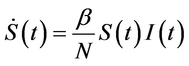
and  the number of individuals belonging to the class S, I, and R, respectively, at time t, the basic SIR model can be resumed in the following three differential equations [6]:
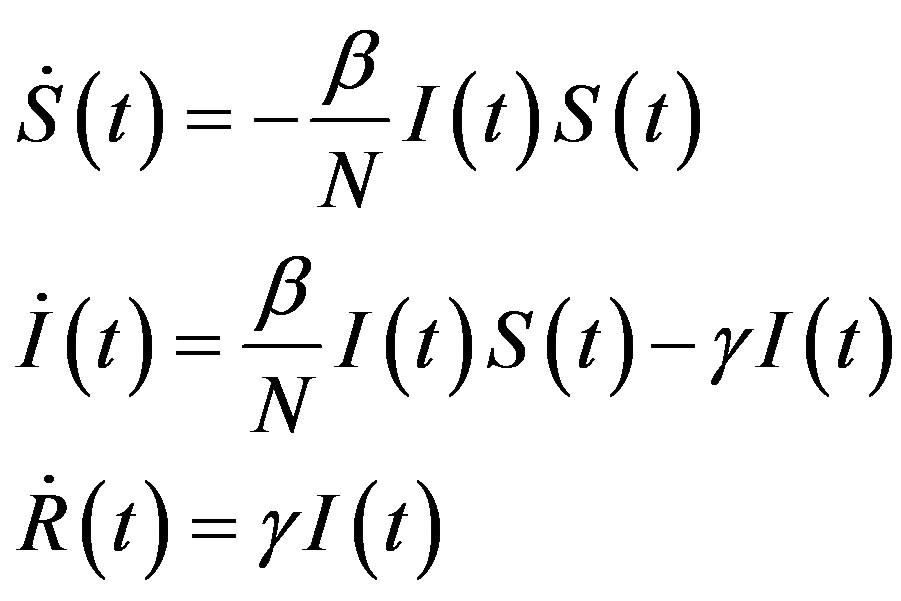 , (1)
, (1)
where the dot represents derivative with respect to time and 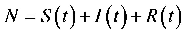 is the total number of individuals in a fixed-sized community and where the parameters are β and γ are the effective infection rate and the recovery rate, respectively. The above set of differential equations can be reduced to two by means of the definition of N given above. Here an exponential distribution of the recovery time is assumed, so that the quantity 1/γ corresponds to the average period which a single individual spends to recover from the illness. Adopting the above description of the time evolution of the number of individuals belonging to the three classes, one can see that an equilibrium point appears in the system if
 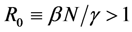 . In the classical SIR model
  is the basic reproduction number, which accounts for the average number of successful contacts an infectious individual has with a susceptible one at the first appearance of the illness in the community.
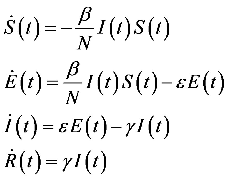
On the other hand, a SEIR model can be represented by the following set of equations [6]:
 , (2)
, (2)
where the exposed (E) class of individuals, whose number at time t is , is added. In this way, assuming an exponential distribution of the quiescent period the inverse of the additional parameter ε represents the average quiescence time of the illness. Notice, finally, that the total number of individuals is now given by
  .
.
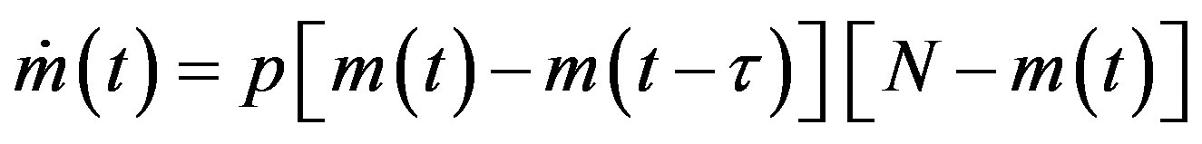
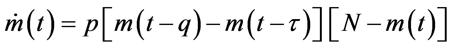
We may notice the nonlinear prey-predator interaction in the first two terms of the above set of equations. The same mass action term is taken to represent the process of infection of the susceptible (S) and the infectious (I) class of individuals in the semi-continuous time delay model by Noviello-Romeo-De Luca (NRD) [7]. In the latter model only one non-linear delay differential equation (DDE) is needed, namely:
 , (3)
, (3)
where  is the count of all illness histories up to time t, starting from t = 0, p is the effective statistical exchange parameter between classes S and I,
  , and τ is the average recovery time. The number of individuals belonging to the S, I and R classes can be found by the following elementary relations:
 , (4a)
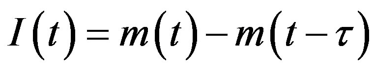 , (4b)
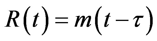 . (4c)
In the present work we extend the NRD model to the case in which a constant quiescence time q is introduced. The effects on the dynamics of the two time-delays τ and q are studied and an approximate solution for the extended NRD model is proposed. A comparison between the classical SEIR model and the extended NRD model is also made.
2. THE EXTENDED NRD MODEL
A detailed treatment of the NRD model can be found in ref. [7]. Starting from a semi-continuous approach, it has been shown that a single globally continuous function  can be adopted to describe the dynamics of all classes of individuals, namely S, I, and R. This model gives good qualitative agreement with existing data on influenza. The recovery time τ in the NRD model is seen to represent a natural time scale and appears as a constant delay time in the nonlinear differential eq.3. Starting now from Eqs.4a-c, in the presence of the additional E-class, we can write:
 , (5a)
 , (5b)
 , (5c)
 , (5d)
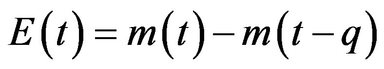
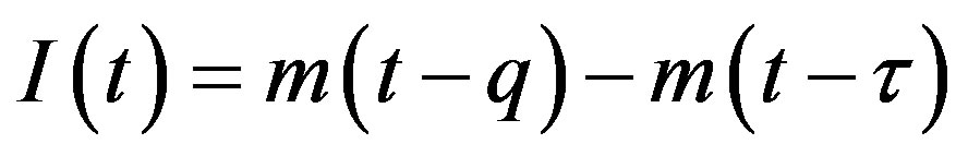
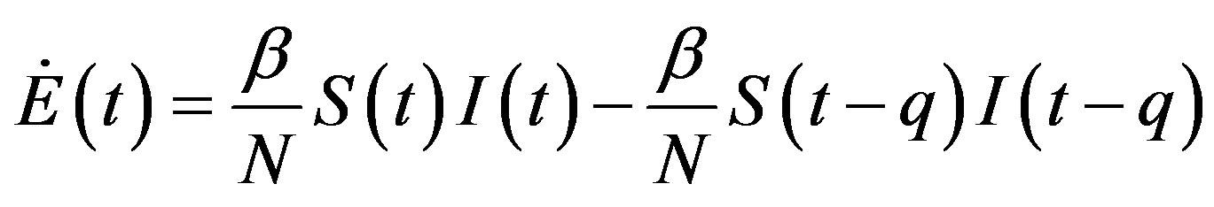
This type of generalization is done by noticing that individuals who have been exposed at time  get ill at time t, while those being infected at time
 , recover at time t. The dynamical equation can thus be written as follows:
 . (6)
. (6)
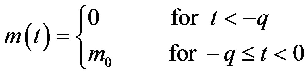
Therefore, in this extended model a second delay time naturally arises and the effective interaction between individuals belonging to the S and I class is modified because of a different expression for  in Eq.5c. Consider q < τ for simplicity, and assume that, at time –q, exactly
  individuals are exposed to infective agents. Therefore, for t < 0, we have
 ,
,  , and
, and
 , (7a)
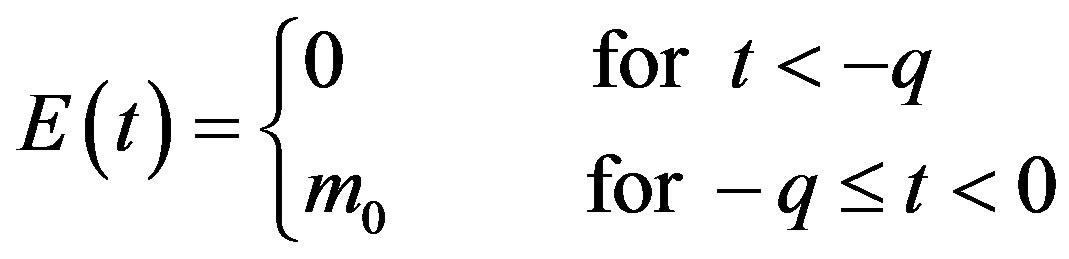 . (7b)
In this way, we have
 . (8)
. (8)
The above relation is needed in specifying the past history of the system, whose dynamics is described by the DDE in Eq.6.
We may notice that the extended NRD model can find application for all those maladies whose characteristics call for well-defined incubation and recovery periods for all individuals in the community. We shall therefore see in details, in the following sections, all peculiar features of the model. We finally notice that the NRD model can be simply obtained from the extended NRD model in the limit q = 0.
3. CHARACTERISTIC FEATURES OF THE MODEL
We have seen, in the preceding section, that the NRD model and its extended version rely upon a single timedelay differential equation, namely, Eq.6. When expressing this equation in terms of the rescaled time variable  and of fractional quantities
  , by defining
 , we may write:
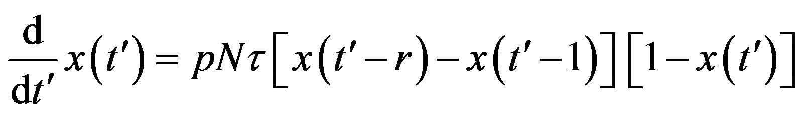 . (9)
. (9)
By defining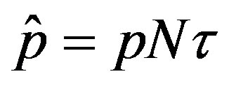 , we notice that the above differential equation can be described in terms of the normalized variable
  of the count of individuals who got ill from the beginning of the epidemic onset, by considering the delay ratio r, the initial value of infectious individuals m0 and
  as the constant parameters of the scalar model in Eq.9. Notice that the quantity
 , by definition, plays the same role as the basic reproduction number R0 in the classical SIR and SEIR models.
In the present work we would like to study the effect of the introduction of the delay ratio r in the DDE (9). At first let us then consider the time dependence of the percentage of infectious individuals obtained by fixing the values of m0 and . In figures 1(a), (b), therefore, we show the numerical solution to Eq.9 for
  and
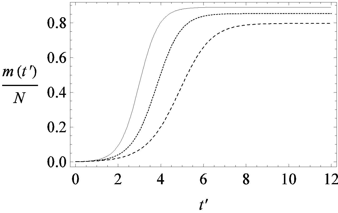
and  and for various values of r. In these curves we notice that, by increasing r from the very low value of 0.01 to 0.5, the total number of individuals
  infected during the epidemic outbreak decreases.
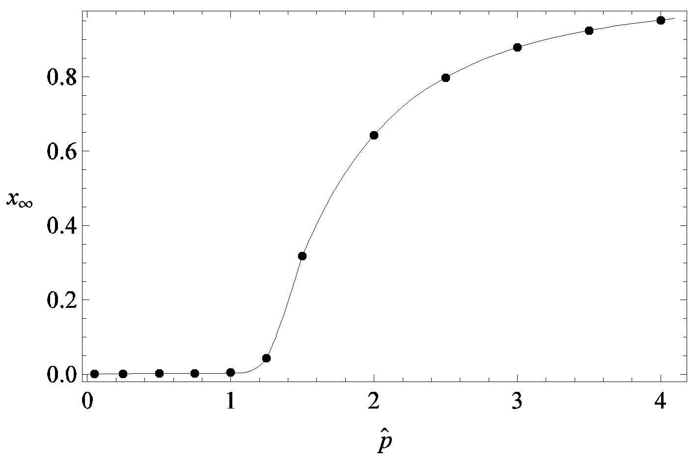
This property is represented in figure 2, where the fraction  is reported as a function of r, the line joining the numerically determined points being a
 (a)
(a)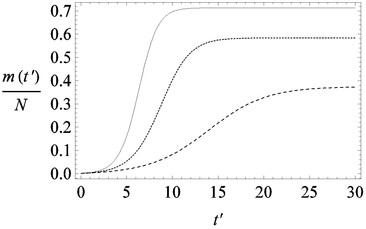 (b)
(b)
Figure 1. Time dependence of the function , normalized to N, for x0 = 0.001 and
  = 2.5, and for: (a) r = 0.001 (full line), r = 0.1 (dotted line), r = 0.2 (dashed line); (b) r = 0.3 (full line), r = 0.4 (dotted line), r = 0.5 (dashed line).
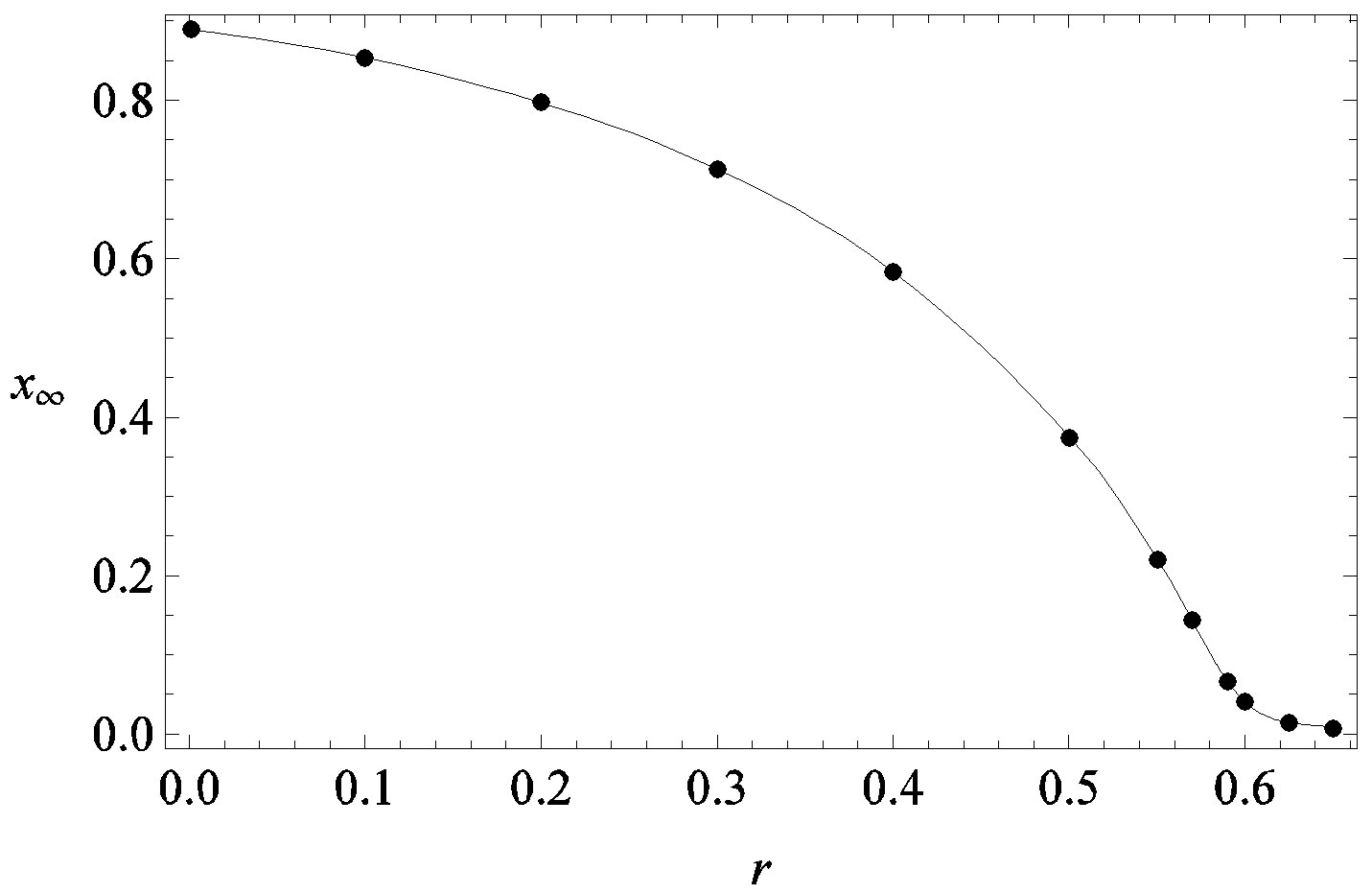
Figure 2. Dependence of the normalized saturation number of individuals getting ill during an epidemic outbreak as a function of the delay ratio r for  and
and  = 2.5. The full line is just a guide to the eye.
guide to the eye. Therefore, one might argue that increasing incubation periods give a minor spread of the disease among the global population. In figures 3(a), (b) we report the time dependence of the fraction  of infected individuals for the same values of parameters as in figures 1(a), (b). The characteristic hump of these curves gets lower and shifts to the right for increasing values of r. In figures 4(a), (b) the onset of the epidemic outbreak can be detected in the curves of the fraction
  as a function of
 .
.
One notices that, below a certain value of , which
 (a)
(a)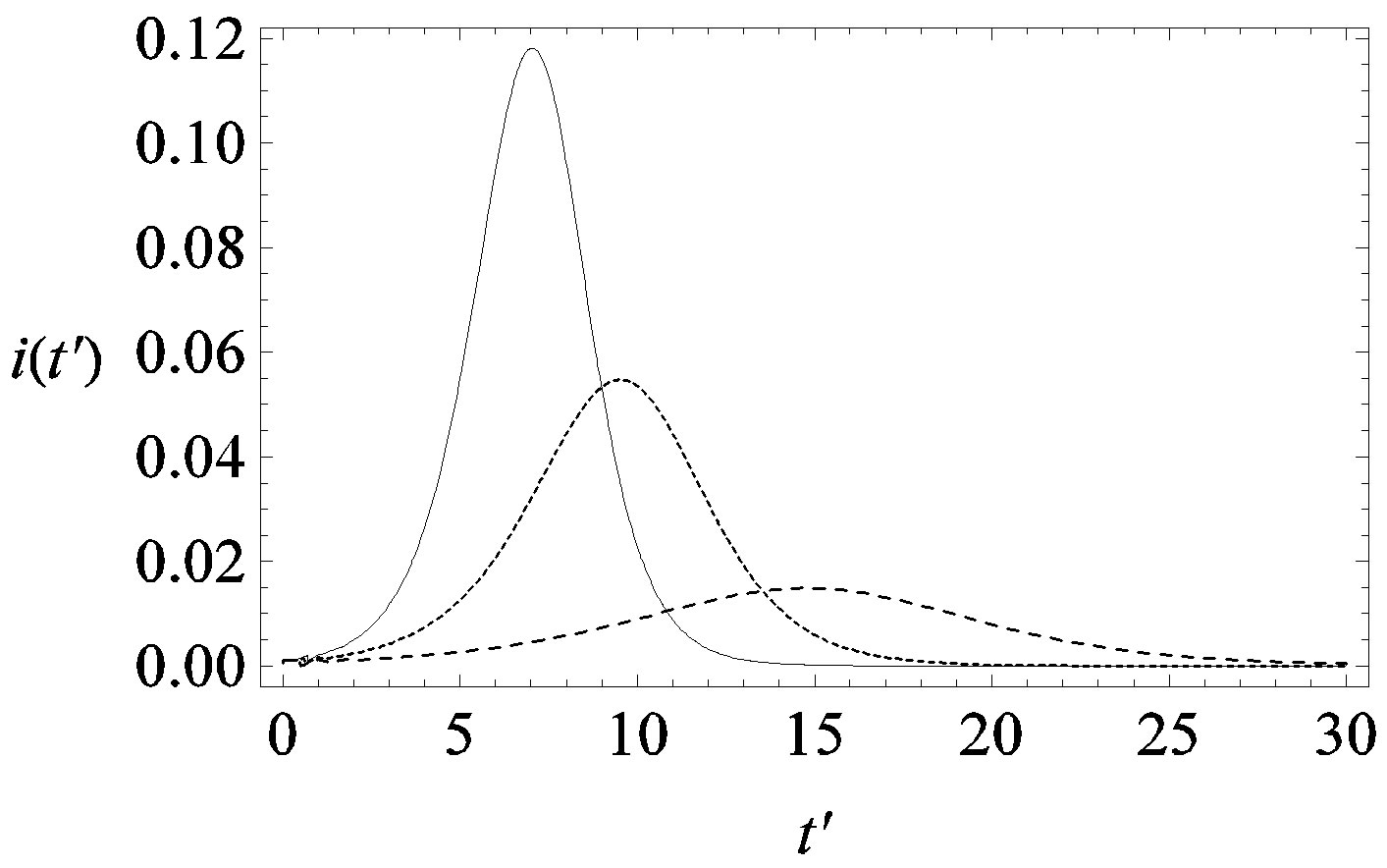 (b)
(b)
Figure 3. Time dependence of the function , number of infectious individuals normalized to N, for
  and
and  = 2.5, and for: a) r = 0.01 (full line), r = 0.1 (dotted line), r = 0.2 (dashed line); b) r = 0.3 (full line), r = 0.4 (dotted line), r = 0.5 (dashed line).
we denote by , the disease is not able to spread significantly among the susceptible individuals, as it happens in the classical SIR and SEIR models. As it appears from figures 4(a), (b), the value of
  is expected to be higher for increasing values of r. Indeed, by collecting points of various critical effective interaction parameter
  for various values of the delay ratio r, we may represent the
  vs. r curve for
  of figure 5. In this plot all points are obtained by defining the onset of the disease in the
  vs.
vs.  curves as the value of
  for which
 . The continuous line is the result of interpolation of the points in the plot, numerically obtained from the
  vs.
vs.  curves, with a trial function
 , with
 . This simple mathematical relation can be understood in the following way. Assuming an increasing behavior for
 , let us write, for reasons which will be apparent in the following section,
  in the limiting region
  , with b arbitrary constant and
 .
.
Assuming an increasing behavior for , let us write, for reasons which will be apparent in the following section,
  in the limiting region
 , with b arbitrary constant and
 . By taking the derivative with respect to
  and substituting this expression in Eq.10, one finds, to first order in
  and
and
 (a)
(a)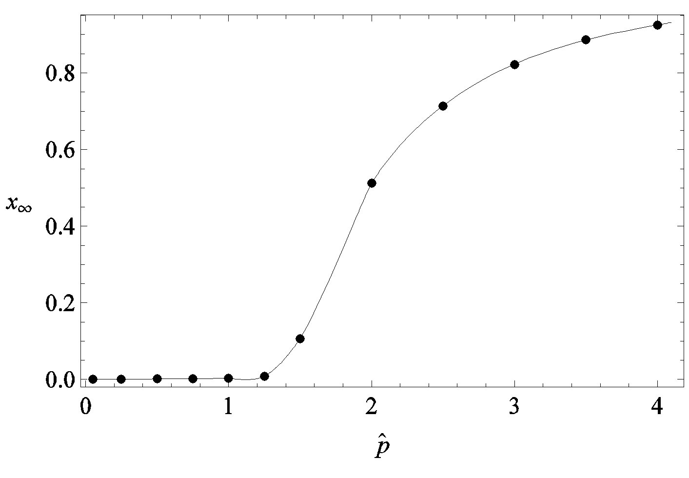 (b)
(b)
Figure 4. Dependence of the normalized saturation number of individuals getting ill during an epidemic outbreak as a function of the effective parameter  for
for  and for delays ratios r = 0.2 (a), and r = 0.3 (b).
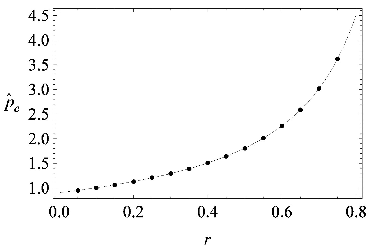
Figure 5. Critical effective interaction parameter  as a function of the delay ratio r for
 . In this plot all points are obtained by defining the onset of the malady in the
  vs.
vs.  curves as the value of
  for which
 . The continuous line is the result of the interpolation of the points in the plot, numerically obtained from the
  vs.
vs.  curves, with a trial function
  with a = 0.9048.
leading order in  a simple expression, expressed term by term as follows
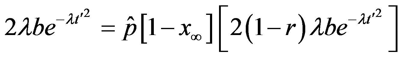 . (10)
In this way, after obvious simplifications, we have:
 , (11)
where
 . (12)
We thus obtain, by this approximate relation, further evidence that the threshold of the infectiveness parameter  increases as r increases as described by the numerical results shown in figure 5.
We can now make a comparison between the dynamics obtained in the extended NRD model and the classical SEIR model. We have already specified that the quantity  plays the same role as the basic reproduction number R0 in the SIR and SEIR models, Eq.12 giving an approximate evaluation of the threshold infectiveness parameter value for the extended NRD model. In the classical SEIR model, on the other hand, the inverse rates
  and
and  corresponds to the average times which a single individual spends in the E or I class, the statistical spread being exponential. The classical SEIR model and the extended NRD model are thus expected to be of different analytical nature, the latter calling for well defined recovery time τ and incubation period q. As an example one can detect this difference in the time dependence of
  curves for both models by setting
  and
and , so that
 , adopting the same values of the parameters
  and
and  and making the correspondence
  for the two models.
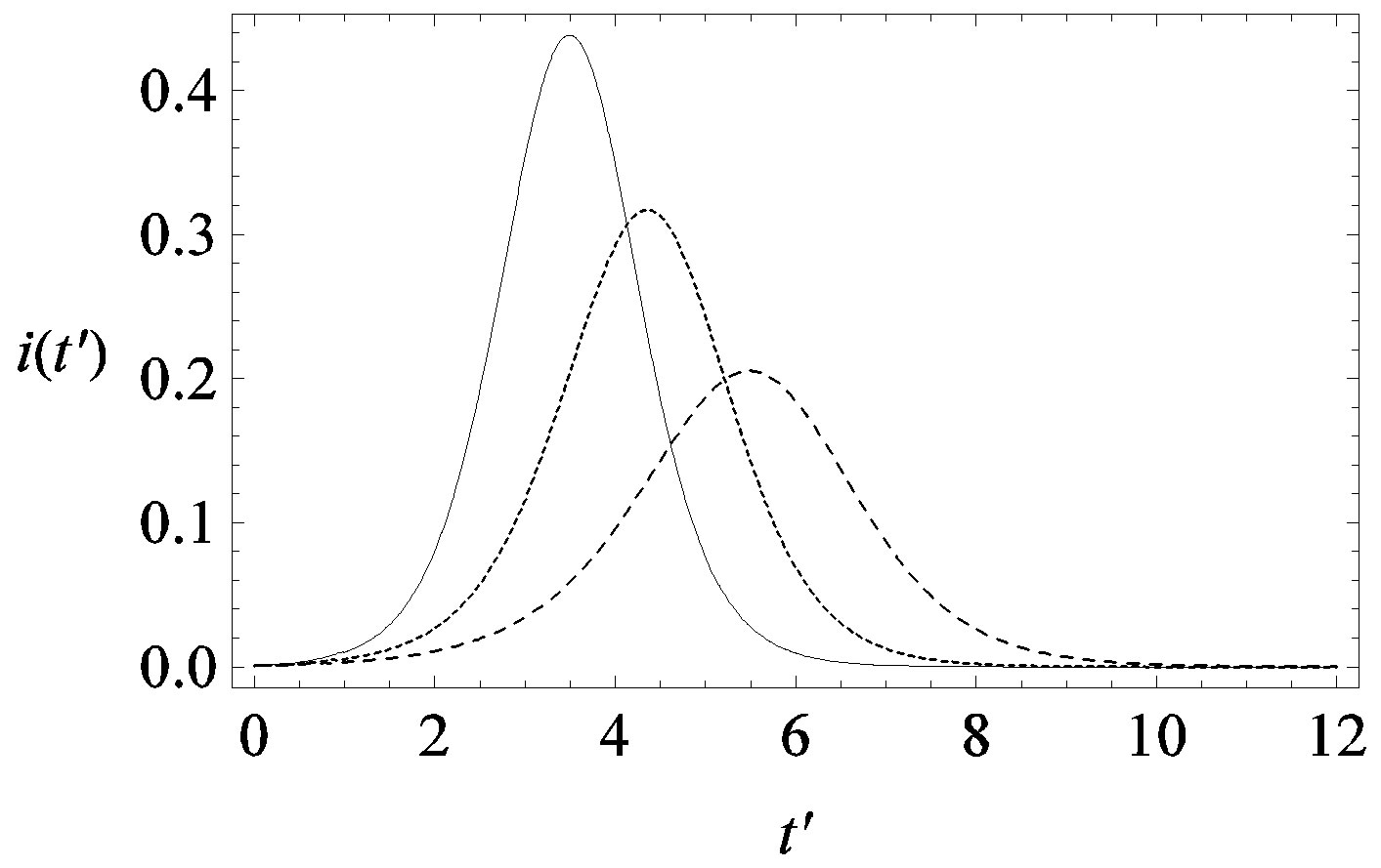
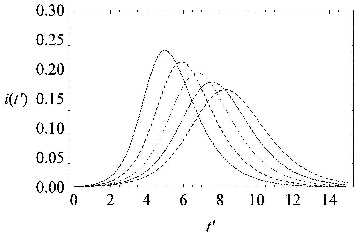
This comparison is very instructive, since it gives a hint on the type of approximation one can make to describe the behaviour of the solution in the asymptotic region, as it has already been done in writing Eq.10. Therefore, in figures 6(a) and (b) we show  curves for the classical SEIR model and the extended NRD model, respectively, for the following values of the delay ratio r: 0.01; 0.1; 0.2; 0.3; 0.4. First of all, we may notice the different pattern in the rise and fall in time of the groups of curves in figure 6(a) and in figure 6(b). This difference and the approximately symmetric pattern about the peak values of the curves in figure 6(b) allow a Gaussian-type approximation of the
  curves obtained for the extended NRD model, as we shall see in the following section. Furthermore, one may also notice a more pronounced decrease of the peak values of the
  curves on increasing the delay ratio r in the extended NRD model, as compared to a correspondingly equal increase of the ratio
  in the classical SEIR model.
Finally, when comparing the classical models with the extended NRD model, it can be useful to notice that the
 (a)
(a)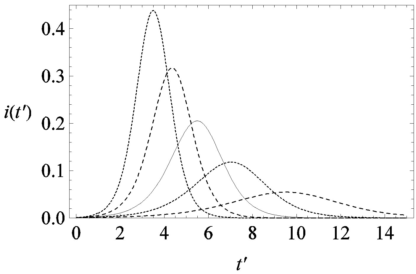 (b)
(b)
Figure 6. Graphical representation of the solution of the fraction of infectious individuals in the SEIR model (a) and in the extended NRD model (b), for ,
,  , and for the following values of r: 0.01 (top dotted line); 0.1 (top dashed line); 0.2 (full line); 0.3 (bottom dotted line); 0.4 (bottom dashed line).
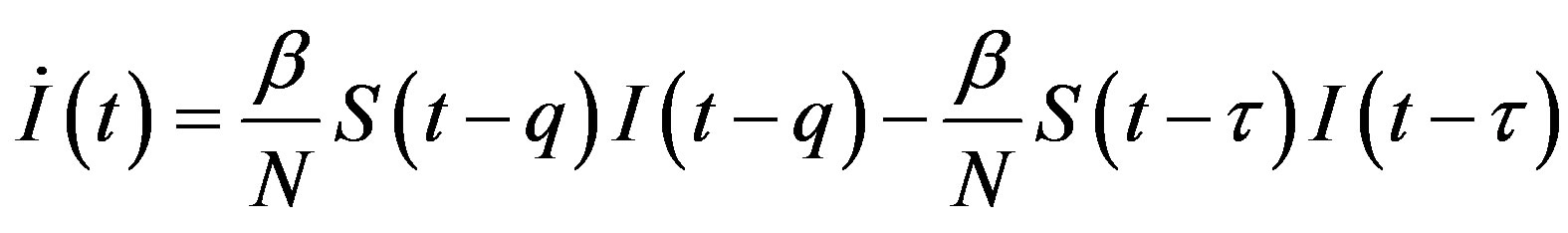
latter generates the delay SEIR model with two constant delays. In fact, by taking the time derivative of Eqs.5a5d and considering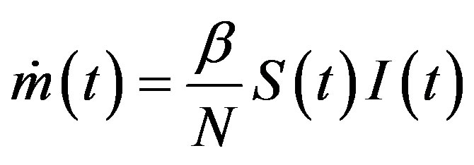 , one can write:
 , (13a)
 , (13b)
 , (13c)
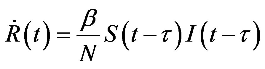 . (13d)
4. APPROXIMATE EXPRESSION FOR THE SOLUTION
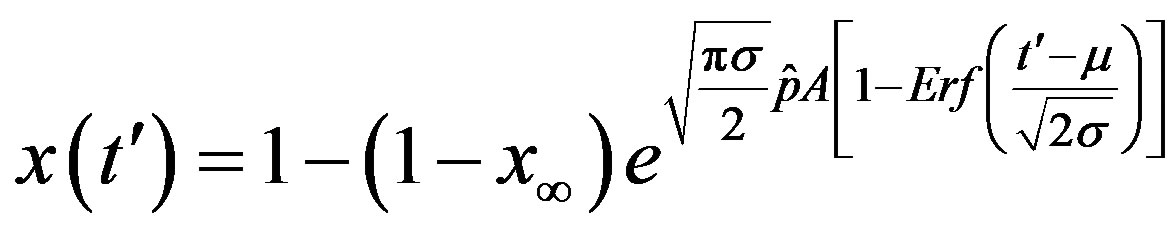
By considering the numerical solutions, shown in figures 3(a), (b), to Eq.10 for , we may consider the following approximate expression for the
  curves
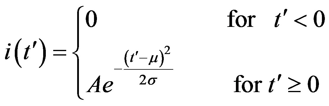 . (14)
where the quantities A, μ, and σ are parameters to be determined. We therefore turn our attention to the dynamical eq.10, which we may approximately write as follows:
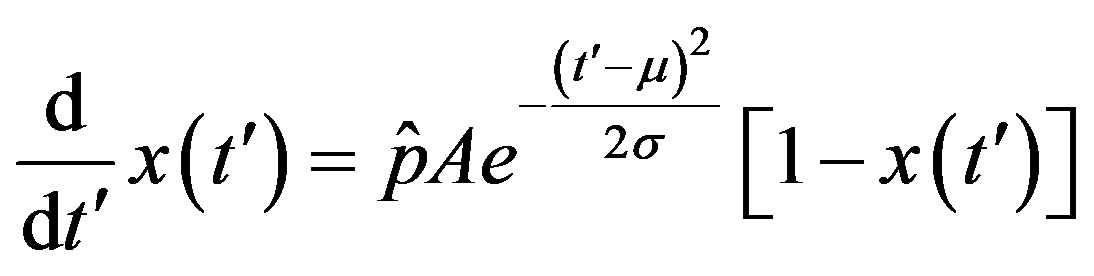 . (15)
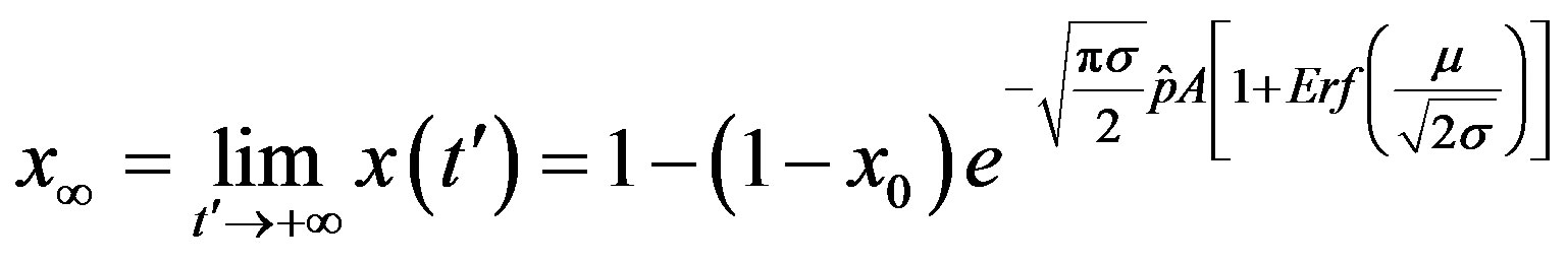
The above ordinary differential equation can be solved by separation of variable for  to give:
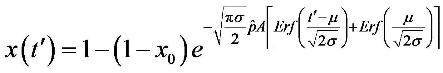 . (16)
where 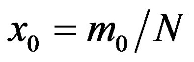 and
and . From the above relation, we find:
 . (17)
In this way, Eq.16 can be written as
 . (18)
A relation between the three fitting parameters can be obtained by considering the definition of  in Eq.5c, by setting
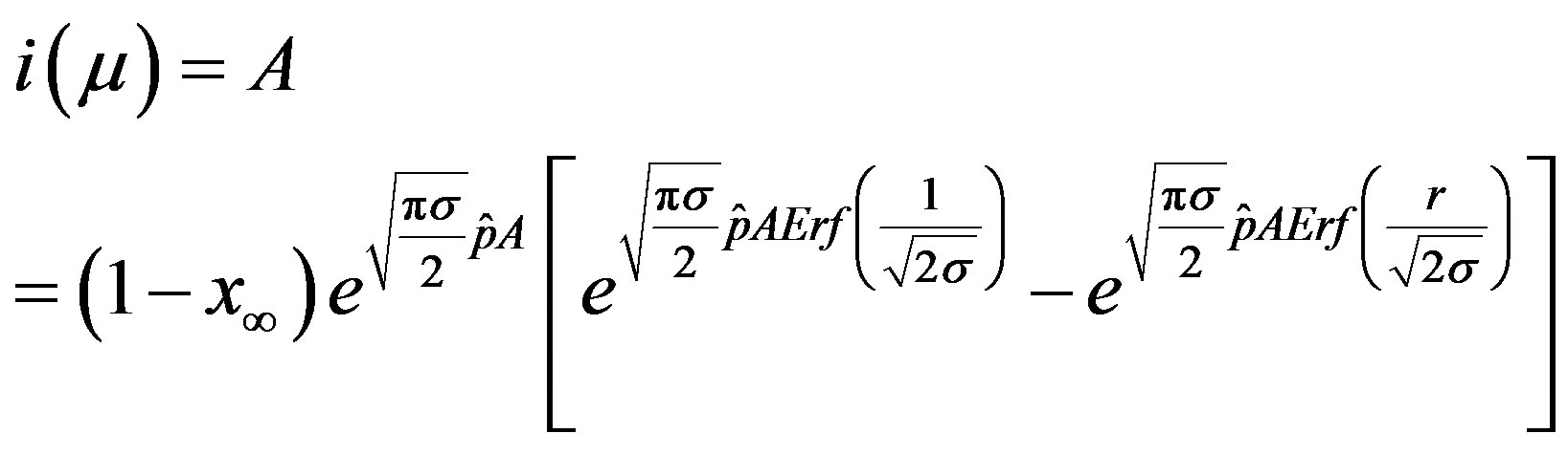 . (19)
The above implicit relation is rather difficult to disentangle analytically to obtain a two-parameter curve for . Therefore, it appears more convenient to keep three fitting parameters in the model. In this way, we find approximate solutions by means of a best fit procedure on the numerically obtained curves shown in figures 3(a), (b), using A, μ, and σ as fitting parameters. In order to fix the ideas, let us start by setting
  and
and . By taking r = 0.1, we find the following values for the fitting parameters:
 ,
,  ,
,
 . Next, by setting r = 0.3, we find:
 ,
,  ,
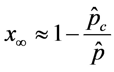
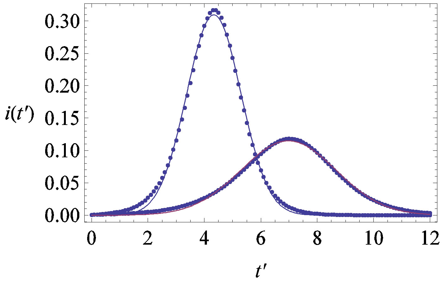
, . The results of numerical integration (dots) along with the approximate solutions (full lines) are shown in Figure 7(a) for these two cases, namely, r = 0.1 and r = 0.3. The curves corresponding to the approximate solution (full lines) of Eq. 10, along with the numerical integration results (dots), are represented in figure 7(b). From the curves shown in figures 7(a) and (b), we may notice the good agreement of the approximate solution in the asymptotic region. However, as already noticed in the previous section, Eq. 12 gives a satisfactory description of the asymptotic quantity
  for which we may write:
 (a)
(a)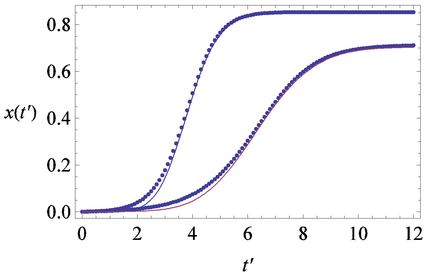 (b)
(b)
Figure 7. (a) Numerical integration (dots) of the  curves for the extended NRD model along with the approximate solution (full lines) for the following choice of parameters:
 , x0 = 0.001, and r = 0.1 (tall curve) and r = 0.3 (shallow curve); (b) Numerical integration (dots) of the
  curves for the extended NRD model along with the approximate solution (full lines) for choice of parameters as in (a), except for the delay ratio, which is taken to be r = 0.1 and r = 0.2 for the upper and lower curve, respectively.
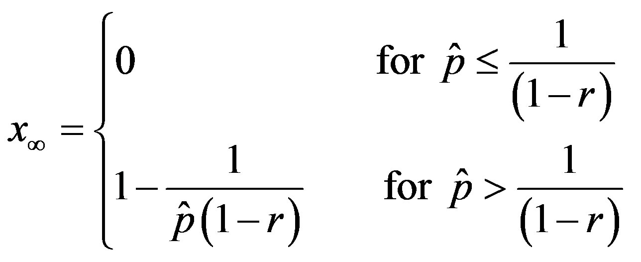 . (18)
The above relation gives similar results to figure 2 and 4 with the advantage of providing a very simple expression for the total number of individuals getting ill during an epidemic outbreak.
5. CONCLUSIONS
The NRD model [7], describing the time evolution of non-lethal infectious diseases in a fixed-size population of N individuals, has been generalized. In the extended version of the NRD model a quiescent time q, in addition to the recovery time τ, is taken as a delay quantity in the dynamics of the infection. The NRD model is recovered from the extended version by setting q to zero.
The influence of the delay ratio  on the model dynamics is studied. It is seen that the model predicts that a longer incubation period mitigates the effects of an aggressive infective agent (
 large). Indeed, as it can be argued from the monotonically decreasing behaviour of the fraction
  of people infected during an epidemic outbreak in the
  vs. r curves obtained for a fixed value of
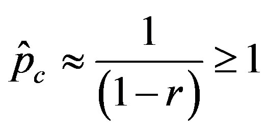
 , the number of total infections decreases as r increases. Furthermore, the critical value
  of the statistical parameter
 , giving the effectiveness of the interaction between susceptible and infectious individuals, is seen to increase for increasing values of r, according to the empirical formula
 , where the quantity a is close to unity and may only depend upon the remaining model parameter
 , which represents the number of infectious individuals at time t = 0. From a comparison between the classical SEIR model and the extended NRD model, one can detect a rather evident symmetry of the latter about a vertical axis passing through the peak values of the
  curves. Owing to these rather simple features, an analytic approximation of the solution of the dynamical equation for normalized variable
  is proposed. The analytic approximation of the solutions to the dynamical equation is shown to be rather accurate in the asymptotic region. Further analytic work is required to investigate the possibility of reducing, in opportune limits, the number of free parameters adopted in deriving the approximated
  curves.
REFERENCES
- Anderson, R.M. and May, R.M. (1979) Population biology of infectious diseases: Part I. Nature, 280, 361-367. doi:10.1038/280361a0
- Anderson, R.M. and May, R.M. (1979) Population biology of infectious diseases: Part II. Nature, 280, 455-461. doi:10.1038/280361a0
- Hyman, J.M., J. Li and Stanley, E.A. (1999) The differential infectivity and staged progression models for the transmission of HIV. Mathematical Bioscience, 155, 77- 109. doi:10.1016/S0025-5564(98)10057-3
- Li, M.Y., Graef, J.R., Wang, L. and Karsai, J. (1999) Global dynamics of a SEIR model with varying total population size. Mathematical Bioscience, 160, 191-213. doi:10.1016/S0025-5564(99)00030-9
- Lipshitch, M.M., Cohen, T., Cooper, B., Robins, J.M., Ma, S., James, L., Gopalakrishna, G., Chew, S.K., Tan, C.C., Samore, M.H., Fisman, D. and Murray, M. (2003) Transmission dynamics of severe acute respiratory syndrome. Science, 300, 1966-1970. doi:10.1126/science.1086616
- Hethcote, M. (2000) The mathematics of infectious diseases. SIAM Review, 42, 599-653. doi:10.1137/S0036144500371907
- Noviello, A., Romeo, F. and De Luca, R. (2006) Time Evolution of non-lethal infectious diseases: A semi-continuous approach. European Physical Journal B, 50, 505- 511. doi:10.1140/epjb/e2006-00163-4