Received 23 December 2014; accepted 6 January 2015; published 19 January 2015

ABSTRACT

As a result of sudden failure in the Programmable Logic Control (PLC) controlled process, the need of diagnosis arises. Diagnosis problem plays an important role to monitor failures in PLC used to control the whole process. Nowadays, due to the lack of the needed tools available to perform this action automatically, it is accomplished manually. Usually, the time consuming method is used by back-tracking the failure on an actuator due to the corresponding sensors. This paper analyzes the software quality metrics and their application on the PLC programs. Aiming to implement metrics that gives predictive information about diagnosability of an Instruction List (IL) PLC programs, this could minimize the needed effort to check the program in case of mistakes. Furthermore, to get a better prediction about diagnosability, new metrics are introduced which are able to give more information about the semantics of a program. But they are not yet fully developed and have to be analyzed.

Keywords:

PLC Programs, Diagnosability, Dependency, Program Slicing Component

1. Introduction

Programmable Logic Controllers (PLCs) are special type of computer with a cyclic behavior used for controlling machines and process. PLC is a good example of discrete event system or logic control with extensions to be able to implement and control analog controllers and deal with continuous signals like PID control algorithms.

The cycle of the PLC starts by reading the sensor values from the controlled process or machine then processing the control algorithm and finally controlling the actuators according to the given specifications.

To maintain the efficiency of the PLC in manufacturing and production, it is necessary in case of modernizations and re-structuring of machines to modernize the PLC to meet these requirements. Another important task related to PLC is the possibility to diagnose the PLC in case of errors or mistaken behavior. Diagnosis is aimed at finding the source of a failure in a system. Many research ideas tackling this problem with advanced methods for failure diagnosis for discrete event systems are available in (‎ [1] - [4] ). Although these methods are rich of research ideas have not yet found wide acceptance in industry.

The standard approach in industry is still manual diagnosis. This is usually performed in case unexpected situation in the manufacturing process. In this case the diagnosis obviously starts by checking the actuator responsible for the missing action. If this actuator is found to function properly, the next step is to back track the reasons through the PLC. The reasons behind this unusual behavior can be because of the non proper or broken sensors. It is generally justified due to the absence of errors in the algorithms implemented on the PLC. Hence, the task is to track back the dependency of the output signal corresponding to the failing actuator―possibly over several internal variables of the PLC―to the corresponding input signals. After these are found, the respective sensors have to be checked for failures. This issue can in turn be very costly and time consuming in case of complex and huge PLC applications.

Fault diagnosis and fault tolerance are important aspects of maintenance which improve the system reliability. These important issues can be implemented in different ways. The main PLCs have self-diagnostic capabilities in order to detect internal failure. Power supply failure is generally shown with a led.

A fault on input/output (units, connecting cable, terminal,…) can be diagnosed with led indicators that show the signal logic value or run specific diagnosis routines.

A run fault (system program termination due to some anomalous operations) is also normally shown with a led.

A complete diagnostic tool within one whole package with the PLC machines or systems is preferable by many testing engineers. However, there’re several tools available, such as:

Ÿ Profibus diagnostic tools;

Ÿ BT200 diagnostic tools from Siemens;

Ÿ xEPI for Ethernet, Profibus, Interface system.

A fault on the application program is more difficult to check, and different solutions have been proposed but not mature. The aim of the presented work is to investigate how to use known software quality measures to determine the connections inside a PLC program. This allows a better understanding of the program and hence the effort for manual diagnosis. The PLC programs under consideration are assumed to be given in Instruction List language (IL). This PLC language is used for the application of the approach because it is the most commonly used PLC language in Europe.

Since IL is a special form of Assembly language, for several metrics to be applied, it is necessary to transform the program to a higher level description. To this end, the presented method utilizes a reverse engineering approach for IL programs presented in ‎ [4] . During the calculation of the metrics graphical representations of dependency relations are derived. These can be used as an aid for the engineer in the actual diagnosis process.

The paper is structured as follows. Section 2 discusses software quality to measure the structure of the PLC program. New methods related to the measures of the dynamic and semantic of a given PLC program are presented in Section ‎3. Section ‎4 concludes this paper and gives and outlook on future work.

2. Software Quality and Diagnosis (Former Works)

In the Software Engineering community, the field of measures or metrics to measure software characteristics is maturing, see e.g. ‎ [5] and ‎ [6] for overviews. Some of the best-known software measures were already date back to the late seventies (‎ [7] [8] ). However, in the area of PLC programs software quality is rarely studied. Frey ‎ [9] introduced the concept of Transparency to measure the understandability of PLC programs described by a special form of Petri Net. Dandachi et al. [10] provided similar metrics to be applied to PLC programs given in Sequential Function Chart language. A different application of software measures is presented by Lucas and Tilbury in ‎ [11] . There, the complexity of solutions to the same problem described with different PLC languages is measured and compared. A systemic method dedicated through the modeling of PLC system architecture and PLC features as components was proposed in [12] and [13] . This model is used for the construction of verification model.

There are many measures which are normally used nowadays to determine the quality of software were applied to investigate the software quality of the PLC programs as Presented in [13] . Most measures presented concentrate more on the program’s structure than on the contents. The size measure belongs to the most often used measures, namely the LOC (Lines of Code) and the Halstead measure with which the software will be measured in terms of the operators and operands. Another classical complexity measure shows the “Cyclomatic Complexity” from McCabe which refers to the flow chart of the code. A measure which determines the complexity of a program by the investigation of its graph is the “Tree Impurity” ‎ [6] .

The following table briefly summarizes the evaluation of the measures presented above and shows their applicability to IL PLC programs (cf. Table 1) ‎ [13] .

3. Code Dynamic and Semantic Measures

3.1. Algorithm to Establish Formulas from IL

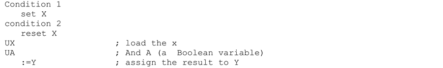
The code is perused from above where the first line of code is processed and the individual conditions according to their operations are recorded. The brackets in the specified conditions are also registered in case available. Each condition has a set, reset or an assignment “i.e.:=”.

IL of the form

The resulting formulas:

(1)

(2)

(3)

The resulting formulas in case of set and reset, for X to be set to 1, the condition to set has to be fulfilled or X

was set to 1 in the previous cycle. To keep X in this state the condition for resetting is not allowed to be fulfilled or X was 0 in the previous cycle. These formulas are used to set X to

1 in case the condition is true otherwise it will be reset to 0.

Set and reset the variable used in the formulas is necessary because by setting a variable it is stored as value 1 or True until the conditions for resetting are met. This can, however, be an advantage to check the programming. When in the formula (i.e. only an X is appeared) which means that for X, the conditions for set or reset is missing. By the assignment operation the processing is different, because no storage for the variable takes place. And the previous state of the variable is not known, this justifies the non-appearance of Y in the formulas.

Once the individual formulas for each variable are constructed, these formulas are substituted into each other and an overall expression for the variables is formulated. If this total expression met, the output variable is set to 1, otherwise it is zero. The above described formulas are expressed with the help of finite state machines (cf. Figure 1 for the first formula, Figure 2 for the second formula, and Figure 3 after the merging of both formulas).

One recognizes here the correctness of the formula, because no matter how many times the loop is executed, the correct output appears accordingly as long as the conditions do not change.

This formula can now be used to determine the software quality of the program. Once you have set all the variables that are represented in the formula for the output calculation, all the variables of which this output depends are obtained. In the formula not only the input variables are yielded, but also it shows which variables are used, such as Merker (used as Flags in Step 5 from Siemens) or other outputs are used to deliver this output. In case outputs or merker from other networks or other function blocks are used, these should be noted using brackets in the used formula. This allows expressing the dependency between the distinct modules. For the software quality, these formulas are used to count the number of outputs and merker. This gives a measure of how far dependency on the individual outputs from each other (cf. Example shown in Figure 4).

Network 1:

Network 2:

After the replacement of A2.5 in A2.4 and A2.6 the Formula for A2.4 become as follows. From the Formula of A2.4 it shows that the output depends on the input variables E6.1; E6.0; E0.2. It is clear that network 2 depends on network 1. The output A2.6 is expressed only one time in the formula which means that the reset condition is not available for this output.

3.2. Dependency Analysis through Program Slicing

In order to prove properties in a program, it is useful to look at only the part of the program i.e. slice, which causes these properties. This slice is then converted into a model in a type of dependency graph ‎ [14] . This graph corresponds to the data flow graph, which additionally edges for paths of all conditions to directly controlled instructions whose execution depends directly on the evaluation of the considered condition inserted [13] - [15] . This provides information on cause-effect relationships in an observed section of the program.

There are two types of a slicing along a dependency graph. The backward slicing, which describes the instructions influence a value under consideration. In a dependency graph all paths that refer to a variable and enter the node are considered. Through this method, irrelevant parts of the program can be hidden during debugging. The forward slicing, describes which instructions are influenced by an observed value. In a dependency graph, all the paths that define a variable in out of a node are considered. Through this slice method the consequence modifications of the program can be estimated ‎ [16] and [17] .

The following summarizes the information available when applying the slicing method:

Ÿ Instructions, which may affect the value of a variable at a certain location under consideration;

Ÿ Involved variables and data flows;

Ÿ Control influences ‎ [6] .

This method shows the dependence of variables has been already transferred to the ladder diagram of PLC in [18] . In this work an algorithm is used to translate the program step by step into a time-machine model by which each conditional statement are assigned to two transitions. The first time automata represent the fulfillment of the condition, which then leads to the next instruction. Other transition is required, if the condition is not satisfied, a negative transition. This then leads directly to the final state of the automaton.

As an application of slicing, data dependency and control can be analyzed on the PLC program. Data dependence and control dependence are known in the literature in terms of the Control Flow Graph (CFG) of a program. CFG is a representation using graph notation which contains nodes representing a basic block without jumps and control predicate in the program, an edge connecting two nodes together which represents the possible flow from former node to another ‎ [19] . Special nodes are used in the CFG to represent the starting and the end of the program labeled START and STOP respectively. The sets of the DEF (i) and REF(i) are used to represent the sets of defined and referenced variables. CFG is used to express several types of dependencies, i.e. flow dependence, control dependence, output dependence and etc. Flow dependence takes place when an instruction depends on the previous instruction, while control dependence occurs when an instruction depends on a preceding instruction to be executed or not.

Program Dependence Graph (PDG) [20] [21] as a slicing methods is used for the reachability. This method can be also applied on the PLC program. PDG is a directed graph with vertices corresponding to statements and control predicates, and edges corresponding to flow and control dependences.

To be able to use these methods of dependency on the PLC program, it should be written on a high level language i.e. Structured Text (ST). Otherwise, if the program is written in IL or any other low level language the Program has to be abstracted first. The abstraction can be applied using the methods and algorithms introduced in ‎ [22] and ‎ [23] . The depicted code in Figure 5 is used to apply the slicing dependency. The program is abstracted using the methods introduced in ‎ [22] and ‎[23] (cf. Figure 6). Figure 7 expresses the CFG, where the edges from the IF conditions to the successive nodes are control dependent, whereas the remaining edges in the figure are flow dependent. Figure 8 elucidates the PDG where thick edges represent control dependence and thin edges represent flow dependencies.

The following table briefly summarizes the evaluation of the measures presented above and shows their applicability to IL PLC programs (cf. Table 2).

4. Conclusions and Outlook

To allow easy diagnosis in the case of failures in a production system automated by PLCs, the quality of the PLC software considered is a crucial factor. As a by-product of the measures calculation several dependence relations can by visualized. It is expected that this will help an engineer in performing the diagnosis task.

The metrics most commonly used nowadays only examine the structure of a program, where it eases the application to the respective programs, as well as on the PLC IL program. They can be implemented directly and provide a rough guideline for the quality of the program. However, the significance of the diagnostic capability with respect to a program could be considered a drawback. It is very difficult, for example, from the length of the code to infer the degree of difficulty of the code.

It is quite different with metrics that focus on the code dynamics. These try to present the relations between individual modules or variables, and thereby find out the complexity of a program. Applying for example the formulas on the PLC, the dependence of the variable, or better expressed: the dependence of the output are determined by the inputs. This gives a better indication than standard metrics, but this is much more difficult to accomplish, because of the effort needed to express the formulas.

The semantic metrics dedicated through the building of the formulas which represent the dependency between the outputs and the inputs in the PLC are investigated. After the building and structuring of all formulas these can be merged together to allow finding the final expressions related to the PLC outputs.

The dependency analysis as a new metric was performed and presented. This analysis explained the best way the variables are changed in a program. In this metric, the dependencies of the entire program were formed. However, these were devoid of information content.

In the next steps, especially the dependency analysis should be further investigated and implemented since through them the best statements about the diagnosability of PLC IL program could be made. Here the focus should be mainly on the slicing, which represents a simplification of the dependence graph by considering only relevant variables for the problem. Once there is an appropriate implementation of the algorithms, it is important to investigate how these models can be used by the inclusion of data models of real plant data for online diagnosis.

References

- Lunze, J. and Schröder, J. (2001) State Observation and Diagnosis of Discrete-Event Systems Described by Automata. Discrete Event Dynamic Systems―Theory and Applications, 11, 319-396.
- Papadopoulus, Y. and McDermid, J. (2001) Automated Safety Monitoring: A Review and Classification of Methods. International Journal of Condition Monitoring and Diagnostic Engineering Management, 4, 14-32.
- Sampath, M., Sengutpa, R., Lafortune, S., Sinnamohideen, K. and Tenekeztis, D. (1996) Failure Diagnosis Using Discrete Event Models. IEEE Transactions on Control Systems Technology, 4, 105-124. http://dx.doi.org/10.1109/87.486338
- Bani Younis, M. (2006) Re-Engineering Approach for PLC Programs Based on Formal Methods. Dissertation, University of Kaiserslautern, Kaiserslautern.
- Höcker, H., Itzfeld, W.D., Schmidt, M. and Timm, M. (1994) Comparative Descriptions of Software Quality Metrics. GMD-Studien Nr. 81, GMD, Bonn.
- Kann, S.H. (2003) Metrics and Models in Software Quality Engineering. 2nd Edition, Addison Wesley Professional.
- Halstead, M.H. (1977) Elements of Software Science. Elsevier, New York.
- McCabe, T. (1976) A Complexity Measure. IEEE Transactions on Software Engineering, SE-2, 308-320. http://dx.doi.org/10.1109/TSE.1976.233837
- Frey, G. (2002) Software Quality in Logic Controller Design. Proceedings of the IEEE SMC 2002, Tunisia, 6-9 October 2002, 515-520.
- Dandachi, A., Lohmann, S. and Engell, S. (2007) Complexity of Logic Controllers. Preprints of 1st IFAC Workshop on Dependable Control of Discrete Systems, Cachan, 13-15 June 2007, 279-284.
- Lucas, M. and Tilbury, D. (2002) Quantitative and Qualitative Comparisons of Plc Programs for a Small Testbed. Proceeding of the American Control Conference, Alaska, 8-10 May 2002, 4165-4171.
- Wang, R., et al. (2013) Component-Based Formal Modeling of PLC Systems. Journal of Applied Mathematics, 2013, Article ID: 721624.
- Bani Younis, M. and Frey, G. (2007) Software Quality Measures to Determine the Diagnosability of PLC Applications. Proceedings of the of the 12th IEEE International Conference on Emerging Technologies and Factory Automation, Patras, 25-28 September, 368-375.
- Horwitz, S., Reps, T. and Binkley, D. (1990) Interprocedural Slicing Using Dependence Graphs. ACM Transactions on Programming Languages and Systems, 12, 26-60. http://dx.doi.org/10.1145/77606.77608
- Weiser, M. (1979) Program Slices: Formal, Psychological, and Practical Investigations of an Automatic Program Abstraction Method. Ph.D. Thesis, University of Michigan, Ann Arbor.
- Weiser, M. (1982) Programmers Use Slices When Debugging. Communications of the ACM, 25, 446-452. http://dx.doi.org/10.1145/358557.358577
- Weiser, M. (1984) Program Slicing. IEEE Transactions on Software Engineering, 10, 352-357. http://dx.doi.org/10.1109/TSE.1984.5010248
- Zoubek, B., Roussel, J.-M. and Kwiatkowska, M. (2003) Towards Automatic Verification of Ladder Logic Programs. Proceedings of IMACS-IEEE CESA’03 Computational, Engineering in Systems Applications, Lille, 9-11 July 2003, 6 p.
- Tip, F. (1994) A Survey of Program Slicing Techniques. Journal of Programming Languages―JPL, 3.
- Kuck, D.J., Kuhn, R.H., Padua, D.A., Leasure, B. and Wolfe, M. (1981) Dependence Graphs and Compiler Optimizations. Conference Record of the 8th ACM Symposium on Principles of Programming Languages, New York, 207-218.
- Ferrante, J., Ottenstein, K.J. and Warren, J.D. (1987) The Program Dependence Graph and Its Use in Optimization. ACM Transactions on Programming Languages and Systems, 9, 319-349. http://dx.doi.org/10.1145/24039.24041
- Bani Younis, M. and Frey, G. (2005) Formalization and Visualization of Non-Binary PLC Programs. Proceedings of the 44th IEEE Conference on Decision and Control (CDC 2005) and European Control Conference (ECC 2005), Seville, 12-15 December 2005, 8367-8372.
- Frey, G. and Bani Younis, M. (2004) A Re-Engineering Approach for PLC Programs using Finite Automata and UML. Proceedings of 2004 IEEE International Conference on Information Reuse and Integration, IRI-2004, Las Vegas, 8-10 November, 24-29.