Journal of Modern Physics
Vol.4 No.8(2013), Article ID:35803,11 pages DOI:10.4236/jmp.2013.48145
A Probabilistic Method of Characterizing Transit Times for Quantum Particles in Non-Stationary States
1Department of Chemistry, Penn State Abington, Abington, PA, USA
2Department of Chemistry, Drexel University, Philadelphia, PA, USA
Email: *kws24@drexel.edu
Copyright © 2013 Hae-Won Kim, Karl Sohlberg. This is an open access article distributed under the Creative Commons Attribution License, which permits unrestricted use, distribution, and reproduction in any medium, provided the original work is properly cited.
Received April 10, 2013; revised May 15, 2013; accepted June 24, 2013
Keywords: Conditional Probability; Non-Stationary Quantum Particle; Transit Time
ABSTRACT
We present a probabilistic approach to characterizing the transit time for a quantum particle to flow between two spatially localized states. The time dependence is investigated by initializing the particle in one spatially localized “orbital” and following the time development of the corresponding non-stationary wavefunction of the time-independent Hamiltonian as the particle travels to a second orbital. We show how to calculate the probability that the particle, initially localized in one orbital, has reached a second orbital after a given elapsed time. To do so, discrete evaluations of the time-dependence of orbital occupancy, taken using a fixed time increment, are subjected to conditional probability analysis with the additional restriction of minimum flow rate. This approach yields transit-time probabilities that converge as the time increment used is decreased. The method is demonstrated on cases of two-state oscillations and shown to produce physically realistic results.
1. Introduction
There are numerous situations where one might be interested in how quickly a quantum particle moves from one place to another. For example, electron transit times may influence such properties as binary switching speeds and alternating current conductance in molecular electronic devices. As another example, when a chemical reaction intermediate is tautomeric, the time required for the intermediate, prepared in one tautomer, to evolve into the other tautomer, may govern the overall reaction rate. In many cases this exchange of tautomers is essentially a proton transfer.
Investigating theoretically the time dependence of a quantum system begins with solving the time dependent Schrödinger equation (TDSE). Solving the TDSE yields the time dependent wavefunction  and the corresponding probability density
 . Consider the movement of a quantum particle between two spatial regions denoted A and B: From the time dependent probability density one may calculate the probability of the particle being in region A at any given time. One may also calculate the probability of the particle being in region B at any given time, but the time dependent wavefunction does not directly yield the time it takes for the particle to travel from A to B. In order to attain quantitative knowledge of the time-dependence of the flow of a quantum particle, it is essential to develop methods to extract this information from the time-dependent wavefunction
  and/or the corresponding probability density
 . Owing to the non-commutativity of the quantum position and momentum operators, the time required for a quantum particle to get from one spatial location to another must be defined differently from the analogous quantity for a classical particle. Here we present an approach that expresses transit time in terms of probabilistic confidences.
To date, the great majority of theoretical treatments of quantum particle flow in molecular complexes have been of the time independent variety. Notable exceptions are Baer’s treatment of anti-coherence in molecular electronics [1] and Pacheco and Iyengar’s demonstration of how to extract the transmission probability from the time-dependence of electron density in donor-bridgeacceptor systems [2]. In related work, Guo has applied non-perturbative time-dependent quantum dynamics to study the phenomenon of superexchange in electron transfer [3], superexchange today being of central relevance in molecular transport junctions [4,5]. Coalson has investigated the accuracy of time-dependent perturbation theory methods to treat nuclear-electronic coupling in long-range electron transfer by benchmarking results for a model Hamiltonian to its exactly solvable limit [6]. Such long-range electron transfer is relevant in a wide variety of donor-bridge-acceptor systems [7]. These studies give insight into the time dependence of electron transfer, but none recover the transit time.
A special case from the class of problems encompassed by the question, “How fast does a quantum particle move from A to B?” is the question of tunneling time through a potential barrier. Tunneling time has been a matter of considerable discussion almost since the inception of quantum mechanics. Valuable reviews have been presented by Hauge and Støvneng [8] and more recently by Winful [9]. The latter review is especially valuable for its appendix, which addresses conceptual questions about tunneling. One issue of sustained interest, apparent superluminal transport across the tunneling barrier, now appears largely resolved [10], as it has been demonstrated that causality is not violated [11,12].
Although we consider a more general problem, the transit of a quantum particle from one spatial location to another, two “tunneling time” papers are more than tangentially relevant to the present work: First, Dumont and Marchioro [13] have given a clear explanation why the question, “How much time does a tunneling particle spend under the barrier?” is ill posed. The difficulty with this question is that its answer would require the simultaneous evaluation of observables corresponding to non-commutative operators. Dumont and Marchioro argue, as we alluded to above, that the question must be posed in a probabilistic manner. Second: Baskin and Sokolovskii [14] addressed tunneling time by generalizing the classical concept of transit time to the quantum mechanical case. We too have found it useful to reference a classical case, but rather than generalizing from a deterministic classical system, we draw analogy to a probabilistic classical system.
In this paper, we present a new way to characterize transit times by analyzing the time-dependent probability density. We then demonstrate the method on the two different systems that display two state oscillations. The movement of the quantum particle is investigated by following the time development of a localized wavefunction, which is expanded in a basis of eigenfunctions of the time independent Hamiltonian using standard methods. From the time development of the wavefunction, we show how to calculate the probability that the particle, initially localized in one orbital, has reached a second orbital after a given elapsed time; or conversely, how to calculate the time that must elapse for the particle to reach the second orbital with a given probability. Collectively, we refer to these questions as the “electron orbital-occupancy problem”. A related question, “How fast can a quantum state change with time?” (under the control of a time-dependent Hamiltonian) is the subject of a work with that title by Pfeifer [15].
2. Two State Oscillations
The time dependence of two-state oscillations is a topic from introductory quantum mechanics. We discuss such oscillations here principally to define the time-dependent probability function for a specific case to be analyzed here, but also to introduce the notation that will be used in the balance of the paper.
Consider an electron that oscillates between two spatially localized states (These localized states could represent the source and drain of a two-terminal molecular electronic device under no applied potential, or the donor and acceptor in a DBA system, but for purposes of this study we consider two generic spatially localized noneigenstates). We want to find out how long it takes for an electron that is initially prepared in one such state to reach a second state. Such a non-stationary state might be prepared with shaped laser pulses [16] or a sudden change in potential [17]. Here we will not concern ourselves with how the spatially localized state is prepared, but rather with how to analyze its time-evolution. To begin the problem we first solve the time-dependent Schrödinger equation (TDSE) by expanding the spatial wave function in a linear combination of eigenfunctions of the time-independent Schrodinger equation (TISE) according to canonical procedure.
Consider a time-independent Hamiltonian  for an electron in which there are two eigenstates
  that obey the relations:
 . (1)
. (1)
The TDSE for this system is:
 . (2)
. (2)
Given that  is time-independent, if we let:
 , then the system separates into time dependent and time independent parts with the solution of the time-dependent part being,
 . Expanding the spatial wavefunction
  in a linear combination of eigenfunctions of
 , it follows that the general form of the solution to the TDSE is,
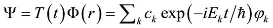 , (3)
, (3)
where the  are the expansion coefficients at
 . Since the basis functions are eigenstates, the probability of finding the system in a particular eigenstate at time
  is,
is, 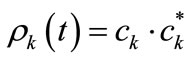 , which is, in fact, independent of time. For our purposes, however, it is more useful to consider an expansion in non-eigenstate functions. For example, suppose that we describe a localized electron in a molecule as an expansion in atomic orbitals (AOs). We can follow the flow of charge by observing how the AO expansion coefficients vary as the time-dependent wavefunction evolves in time. Ultimately, we want to address the question; how long does it take for an electron that is initially localized in one AO to reach a second selected AO?
Suppose that the two eigenstates ( and
and ) of the two-state system are expanded in a basis of two AOs;
  and
and . In this basis, the TISE in secular form is,
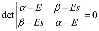 (4)
(4)
where ,
,  , and
, and . The solutions are,
 (5a)
(5a)
 (5b)
(5b)
If we use the approximation,  , the roots are,
 . (6)
. (6)
Both eigenvalues are displaced from the site energy  by an amount dependent on the coupling matrix element
 . Since
  just sets the zero of potential, we can take the eigenenergies to be
 .
.
Suppose that we initially localize our electron by placing it exclusively in the AO . At
. At  the spatial wavefunction, written as an expansion in AOs, is,
 . (7)
. (7)
To write the time-dependent wavefunction, we must express this in the basis of eigenfunctions of . In other words, we must find the
  in Equation (3). This is a standard change from an AO basis to a molecular orbital (MO) basis. From the definitions of
  in Equations (5a) and (5b), it follows that
  and
and .
.
We can now write the time dependent wavefunction:
 (8)
(8)
To follow the time evolution of the wavefunction in space, we need to transform from the MO basis back to the AO basis. Using the Euler relations, we obtain the time dependent AO-occupancy probabilities as:
 (9a)
(9a)
 (9b)
(9b)
As expected, . Note that the frequency of oscillation between the two functions is
 . Note also that the oscillation frequency depends on the energy difference between the states, the greater the energy difference, the greater the frequency.
In oscillatory systems the period of oscillation  bears a reciprocal relationship to the frequency
  where
where  is the angular frequency. As shown in the example above, a bound quantum system in a non-stationary state is characterized by such a frequency, (or frequencies in a system with more than two levels). The related period(s), however, is(are) a physically unsatisfactory metric of the lifetime of the associated spatially localized state. In Section 5 we demonstrate that this quantum exchange frequency suggests a rapid exchange between tautomers in cases when one would likely have to wait an aeon for one tautomer to evolve into another. The present paper addresses this dilemma.
Solution of the TDSE as outlined in this section yields the time-dependence of occupancy for each spatially localized orbital (AO). This standard procedure is easily generalized to an arbitrary number of AO basis functions. It is a standard result in quantum mechanics and answers the question, “what is the probability that a selected AO is occupied at a specific time t?” Herein we will demonstrate how to analyze the time dependent probability function to address our central question: Given that the electron is initially localized on one atomic orbital, how much time must elapse for the electron to reach the second orbital with a given probability? In the next section we look at an analogous classical system in order to develop the methods to answer this question. The system we look at is a “professor office-occupancy problem”.
3. Professor Office-Occupancy Problem
To develop the methodology, we first consider a classical problem analogous to the “electron orbital-occupancy problem”: We ask the question; given a function that describes the probability of a professor being in her office as a function of time, what is the probability that the professor has occupied her office at least once during some elapsed time period? We term this the “professor office-occupancy problem”. Exploration of this classical problem allows us to identify the variables that are important in the electron orbital-occupancy problem and to determine what assumptions might be necessary to produce a physically reasonable answer. Our approach is based on evaluating the time dependent probability density  at a fixed time increment. We find that conditional probability analysis is required to obtain a result that converges as the time increment is decreased. The understanding gained from studying the professor office-occupancy problem is then applied to solving the electron orbital-occupancy problem. In addition to studying the time dependence of electron orbital occupancy, the method is also demonstrated for proton exchange in a double well potential.
The professor office-occupancy problem is defined as follows: We take the probability of finding a professor in her office,  , to be a sinusoidal function of time with a period of 24 hours and an amplitude of 0.79; a minimum at midnight at which there is 1% probability of finding her in her office; and a maximum of 80% probability at noon. The function is shown in Figure 1 (In this analysis we assume all days, whether weekend, weekday or holiday, are equivalent. A more complicated function with 7-day or 30-day periodicity could be used, but this would only serve to obfuscate the analysis without introducing any new physics). The probability function may be written as,
 , (10)
where  is time in hours. The area under the curve, 9.72 hours/day, is the average amount of time the professor spends in her office each day.
This system can be thought of as a two-state oscillation. The professor is either “in” her office or “not in” her office, and she oscillates between these two “states” according to the assumed probability function (10). Now let us address the question; given a specific start time, how much time must elapse for the professor to have visited her office at least once with a selected probability? One way of thinking about the question is this: If a student comes to the professor’s office, how long must the student wait to be 90% confident (or 99.999% confident) that the professor will show up?
The student could show up at the professor’s office and wait. Alternatively, the student could check the office periodically. As the frequency with which the student checks the office approaches infinity, the elapsed time to finding the professor must converge to the period
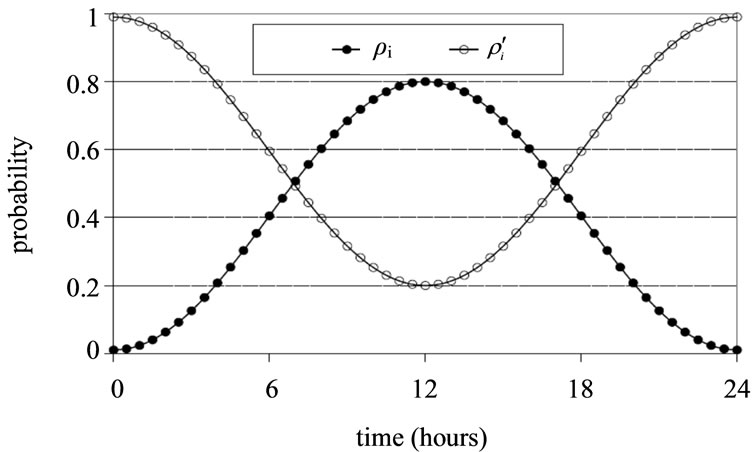
Figure 1. Probability  of finding a professor in her office as a function of time together with the probability
  that the office is not occupied.
of time the student would have to wait at the office door. Convergence of the time to achieve a given confidence level with increasing sampling frequency is therefore a necessary condition for the validity of any approach that is based on repetitive sampling of the probability function. In the next subsection we show that simple multiplication of the probabilities extracted from the probability function fails in this regard.
3.1. Simple Probability Analysis
We begin our analysis of the professor office-occupancy problem by studying what happens if the student checks the professor’s office periodically. The naive approach assumes probabilistic independence, in which case the probability that the office has never been found to be occupied in  samplings
  is,
is,
 , (11)
where  is the probability of the office being occupied in a specific sampling event
 . The probability that the professor has been found in her office is then
 . This approach may appear to give reasonable results for widely separated sampling events
 , but obviously the assumption that
  and
and  are probabilistically independent is flawed. Consequently, the method fails as
 . This failure can be seen by considering four cases: 1) The student looks for the professor at exactly noon each day. 2) The student looks for the professor at noon and midnight each day. 3) The student looks for the professor at noon and 2 seconds after noon each day. 4) The student looks for the professor at noon and every 2 seconds thereafter until 12:00:08 pm each day.
Applying Equation (11) to the four cases described above yields the results in Table 1, which shows the day on which the probability of having found the professor exceeds 99.999%. In case 1, after  consecutive days the probability that the student has located the professor is
 . This expression converges to 1.0 with increasing
 , a physically sensible result. In case 2, after
  consecutive days the probability that the student has located the professor is
 . This converges to 1.0, but slightly more rapidly than if the student checks only at noon, again a physically sensible result. By checking at midnight in addition to noon, the student increases the probability of finding the professor, but only by a little because the professor is very unlikely to be found in her office at midnight.
For case 3, since
 after
after  consecutive days, the probability of having located the professor will be
 . This result is
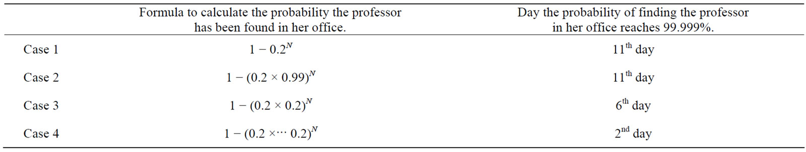
Table 1. The day the professor is found in her office with 99.999% probability, based on looking for her at different times of the day under the assumption that these samplings possess probabilistic independence.
completely unreasonable. The probability is converging to 1.0 more rapidly than in case 1, only because the student is making two attempts to find the professor at essentially the same time each day! Case 4 further highlights the failure of this approach. Table 1 shows that the professor is found 10 days earlier simply because the student is looking into the office every two seconds for 8 minutes each day, instead of simply checking once.
The reason for the failure of Equation (11) is that  is very strongly correlated to
  for small
  owing to the continuity of the time evolving probability function
 . In the next section we describe an approach that accounts for the correlation between sampling events to produce a predicted time to achieve a given confidence level that converges with increasing sampling frequency.
3.2. Conditional Probability
During a discrete time-step , the condition of the professor being in the office will either change or stay the same. In general, the probability that the condition changes may depend on the initial state. We can represent the evolution during a time‑step with a tree as depicted in Figure 2.
In the tree diagram,  is the probability that the “state” changes given that the professor is not in her office and
  is the probability that the state changes given that she is in her office (
 and
and ). We can write the probabilities of being in the office at
  as:
as:
 , (12a)
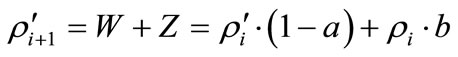 . (12b)
If  and
and  can be determined from
  and
and  (and
(and  and
and ) it is then possible to determine the probability that the professor was never in her office. The probability is given by the probability that the office was not occupied at time
  times the probability that the state did not change on each subsequent time-step
 . In other words, given that the office was not occupied at time
 , if the probability that the state did not change between time
  and time
  is
is
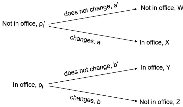
Figure 2. Conditional probability tree diagram where:  is the probability that the professor is in her office at time
 , is the probability that she is not in her office at time
 , and
, and , at any time
 .
.
given by , then the probability that the office was never occupied is given by,
 . (13)
In fact, Equations (12a) and (12b) are dependent and we can therefore only solve for  in terms of
 . While a definitive relationship between
  and
and  is not obvious, both
  and
and  values must be confined by
  because they represent probabilities. By rearranging Equations (12a) and (12b), we obtain the following expressions.
 (14a)
(14a)
 (14b)
(14b)
Using probability function Equation (10) and the relationships of (14a) and (14b), we can find the range of allowed values of  and
and  at each time-step.
Consider as a specific example, the set of conditions: ,
,  ,
,  ,
, . It follows that for this specific set of conditions,
 . (15)
We haven’t identified another relationship between  and
and , but we do know that
  and
and . The range of allowed values of
  and
and  for this example case is shown with the boldface line segment on the LHS graph of Figure 3.
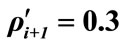
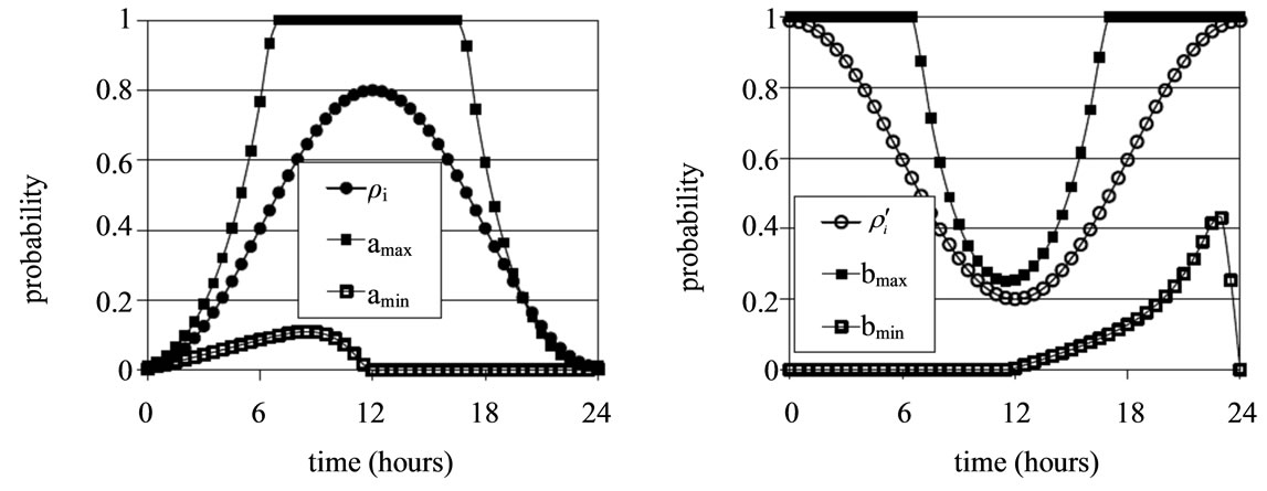
Based on analyzing the allowed ranges for  and
and , the minimum and maximum allowed values of
  and
and  using two sampling timesteps, (0.5 hour and 0.1 hour) are shown in Figures 4(a) and 4(b). From the figures we see that
  and
and  decrease as the time-step gets smaller. This is a physically sensible result: As the time step decreases, the probability that the state changes during the time step also decreases (i.e., the state is very unlikely to change during a very short time interval).
There are many mathematically allowed solutions of Equation (14) for  and
and . To obtain the physically meaningful solution, a second condition on
  and
and  is required. One obvious possibility is
 . Using this condition, direct application of Equation (13) produces the same unphysical result as the simple probability approach. The predicted time to achieve a given confidence level does not converge with decreasing time-step. We conclude that this obvious additional condition on
  and
and  is not the physical one.
We note that physically,  and
and  represent the probabilities of the “occupied” and “unoccupied” states changing during the given time interval. While we do not know the specific values of
  and
and  for any given
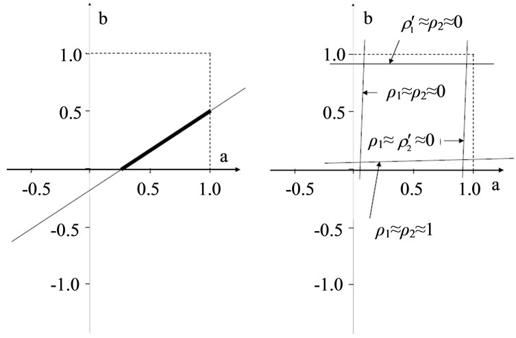
Figure 3. LHS: allowed ranges for  and
and  for the set of conditions:
 ,
,  ,
,  ,
, . RHS: extrema of allowed values of
  and
and  in general.
 (a)
(a) (b)
(b)
Figure 4. (a) Allowed range of  and
and  values for conditional probability for professor office-occupancy problem. Also plotted are the
 , with
 ,
,  and
and  with
with ,
, . The plots are made for 0.5 hour time intervals. (b) Allowed range of
  and
and  values for conditional probability for professor office-occupancy problem. Also plotted are the
 , with
 ,
,  and
and  with
with ,
, . The plots are made for 0.1 hour time intervals. The spacing of data points is so small that individual points have been replaced with an interpolating curve for visual clarity. Note that
  and
and  are smaller than in Figure 4(a) where a larger time step was used.
time interval, it is physically reasonable that as the time step is decreased, the probability of the state changing during any one time step decreases. In the limit of decreasing time step therefore,  and
and  should take on their smallest allowed values. We therefore used the slowest mathematically allowed flow of probability by using
  where we denote
  and
and . The case
  represents the fewest office occupancy state changes that produce
  and
and , from
  and
and . This is the physically meaningful additional condition on
  and
and .
.
In the range , the probability that the office is occupied is increasing, therefore the minimum change is accomplished by setting
 , which produces
 . Here, if the office is occupied it remains so, if it is not, there is a small probability of a change in the state
 . Similarly, for
 , the probability that the office is occupied is decreasing. The minimum change is accomplished by setting
 , which produces
 . In this case, if the office is empty it remains so, but if it is occupied there is a small probability of a change in the state
 .
.
One might argue that the state of the system could change during the first time interval (or any subsequent time interval) regardless of how short the time increment is, in which case , not its minimum allowed value. This is true, however, we seek to place a confidence on the office occupancy within some elapsed time. While the rapid state change may happen, to specify a confidence that the state change has happened we must base our analysis on the slowest rate of state change that is consistent with the probability function.
Using the above analysis, we can put rigorous upper and lower bounds on the flow of probability. To obtain the upper limit, we use . In this case the office is occupied the first time we look. To obtain the lower limit we use
 , which produces
  as shown in Figure 5. Note that
  drops below 0.1 at 30.5 hours.
(Half-hour time steps were used to generate the figure). This is the elapsed time at which we can be 90% confident that the professor has been in her office at least once.
The results (collected in Table 2) show that as the time-step gets smaller, the approaches using simple probability, and conditional probability using , predict that the time to 90% occupancy probability decreases to zero with increasing sampling frequency, a physically nonsensical result. Only the conditional probability analysis with the assumption of minimum flow produces a result that converges.
3.3. V alidation by Monte Carlo Simulation
3.3.1. Simulation Methods
To validate our findings, we performed Monte Carlo (MC) simulations based on the time-dependent probability function (10) for both the simple probability and conditional probability approaches. We compared the results to direct application of equations (11—simple probability
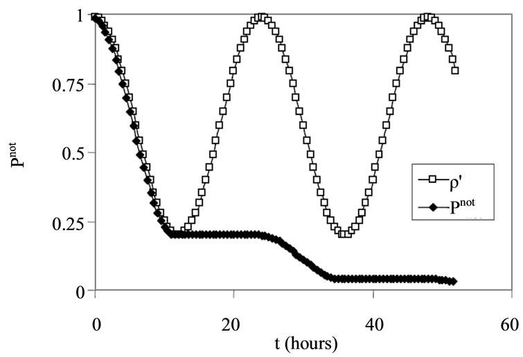
Figure 5. Time dependence of  (the probability that the office is not occupied) and
  (the probabilistic confidence that the office has never been occupied between
  and
and  ) based on conditional probability analysis.
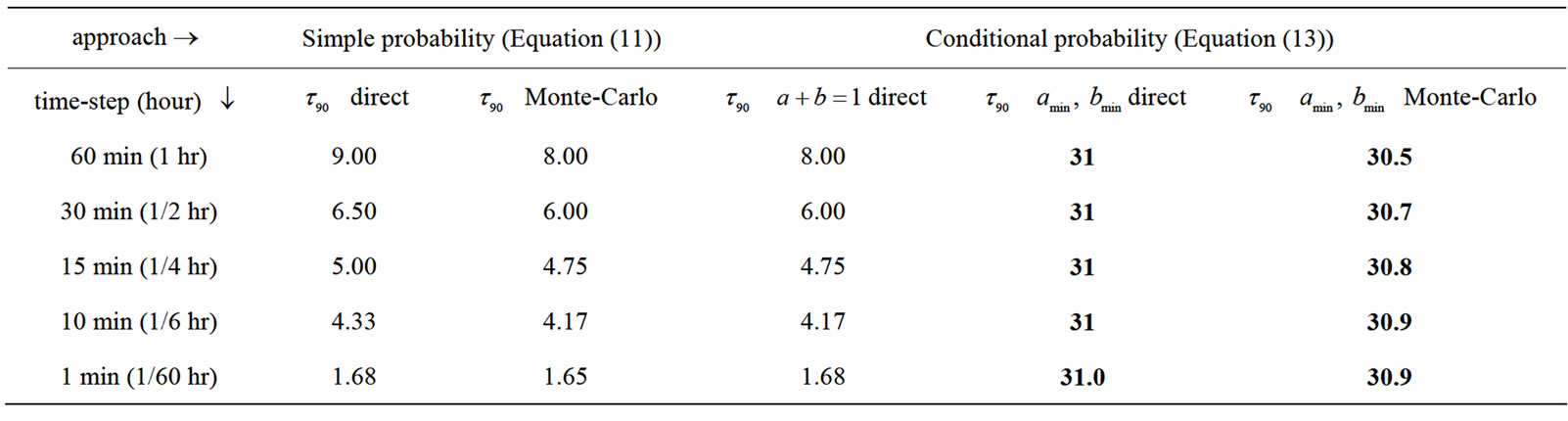
Table 2. The elapsed time (hours) at which the professor is 90% likely to have been in her office at least once . The boldface result is the physically meaningful one. The other results are based on the flawed assumption that samplings of the probability function are independent events. Monte-Carlo denotes the result of a Monte-Carlo simulation. Direct denotes direct application of the noted equation.
analysis) and (13—conditional probability analysis). For consistency, in all cases we determined the elapsed time when the professor is 90% likely to have been in her office at least once .
.
In the first set of MC simulations, (simple probability) the “1st visit time” is found by starting at time  of the first day and advancing in discrete time steps
 . At each time-step a random number is chosen between 0 and 1. If the random number falls under the probability curve
  the professor is taken to be in her office and the answer is obtained. If the random number falls on or above the curve, another time-step is taken and so on until we get the 1st visit. We look at all first visits and find the time of day when 90% of the first visits have occurred. We continued to follow the professor’s movement beyond the 1st visit to validate whether the simulation procedure reproduces the
  profile. (This allows us to look at the office-occupancy problem without an artificial day-cycle boundary.) One or multiple consecutive in-office-states constitute a single visit. Most of the visits are in the middle of the day-cycle as expected. This approach reproduces the
  profile with the professor spending on average 9.72 hours per day in the office as shown in Figure 6.
For comparison, for direct application of Equation (11), the time the professor is found in her office at least once with 90% probability is determined by setting the value of Equation (11) to 0.1 and solving for . Here
  runs from 0 to
  and
and . The probability is given by the probability that the professor was not in her office at time
 ,
,  times the probability that she was not in her office at the end of each subsequent time-step
 . The product is carried out stepwise, incrementing N by 1
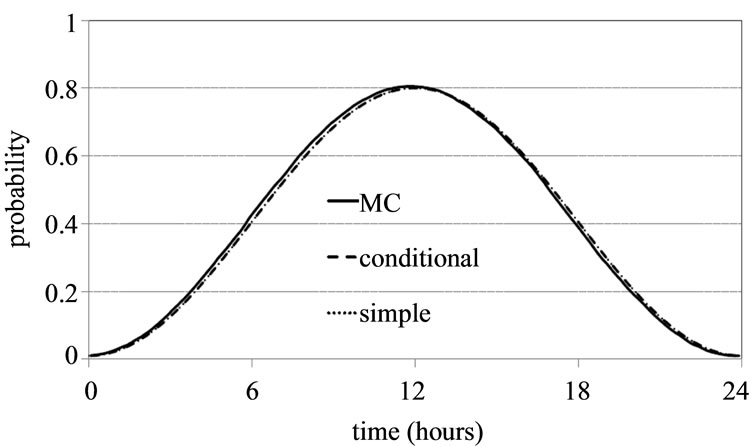
Figure 6. Comparison of  profiles based on simulations with
  function of Equation (1): MC = MonteCarlo simulation, conditional = simulation with conditional probability with minimum flow, simple = simulation based on simple multiplication of probabilities. For the MonteCarlo simulations 10,000 day-cycles were used. All of the simulations reproduce the original
  function and predict an average of 9.72 hours spent in office per day.
until  drops below 0.1.
A Monte Carlo simulation based conditional probability with minimum flow is obtained in a very similar manner as the simple probability approach described two paragraphs above, but with one difference; at each timestep we compare the random number to the  in the range
  and
and  , for the range
 , instead of comparing the random number to
  as done in the simple probability approach.
Direct application of Equation (13) was accomplished analogously to direct application of Equation (11). This product, and all other simulations described in this manuscript, were carried out using program MATLAB [18].
3.3.2. MC Results
In Table 2 we report the results of our calculation using varying time-steps. The results show that the answer given by the simple probability approach depends on how frequently the office is checked and converges to zero as the time step is decreased, a physically nonsensical result. Simply checking the office with infinite frequency does not guarantee that the professor will arrive immediately!
As shown in Table 2, the simulation based on the condition of minimum flow produces an answer that is independent of time-step and is exactly the same as the analytic analysis shown in Figure 5, and the direct application of Equation (13). The minimum flow conditional probability approach also produces the correct  profile as shown in Figure 6 with a total office time of 9.72 hours per day-cycle.
In the approach using conditional probability with minimum flow rate, since  from noon till midnight, no first visits are found during the final 12 hours of a day-cycle. As a result, some days have no visits at all and the answer, time ‘till the first visit, is greater than 24 hours (It is important to note that the professor can arrive at her office within the first 24 hours, or 12 hours or any shorter time interval, but 90% confidence is not achieved until later). This approach achieves our requirement of obtaining a solution to the problem that converges with decreasing time-step.
There is an important feature of quantum mechanics that merits note here: In a quantum system, the timedependent wavefunction (and its corresponding probability density ) evolves according to the TDSE until the state of the system is observed, whereupon the system collapses into a stationary state. In practice therefore, the process that we draw analogy to, systematically and repeatedly peeking into a professor’s office to ascertain its occupancy, would function for that classical case, but not for a quantum mechanical system. In a quantum system, the first such “measurement” would collapse the wavefunction into a stationary state. It is important to draw a distinction, however, between carrying out a measurement of the system and evaluating a probability density function. To analyze the mathematical properties of
  we may evaluate it at numerous values of
  without altering the function, just as integrating the absolute square of a 1D spatial wavefunction
 over the interval
  to establish that it is properly normalized does not collapse the system into a single-valued position state, which would be represented by a delta function. For this reason, we may use the analogy to the classical office occupancy case to inform us of how to analyze the time evolving probability function. In the ensuing sections we apply the minimum flow conditional probability analysis to two quantum mechanical systems.
4. Electron Orbital-Occupancy
We have applied the methods developed above to the orbital-occupancy problem where  gives the time dependence of electron occupancy for orbital
  (See Equation (9b)). The oscillation frequency is
 . In our calculations we took the values of
  and
and  to be 1. The cycle length is therefore
  (The function repeats every time
  advances by
 ). The results of our studies for the electron orbital occupancy problem are collected in Table 3, which shows the elapsed time (fraction of a cycle) at which the electron is 90% likely to have occupied the second orbital at least once. Note that just as in the professor office-occupancy problem, the simple probability approach produces the physically unreasonable prediction that as the sampling rate increases, the time to 90% occupancy probability converges to zero. The simple probability and
  Monte Carlo simulations produce the same unphysical result because they are based on the same flawed assumption of uncorrelated probabilities. The approach of using conditional probability with minimum flow rate converges to 1.25, indicating that at about 125/314th of an oscillation cycle, the electron has reached the second
“acceptor” orbital with 90% probability.
While the results presented here employ a basis of two atomic orbitals, the extension to a larger basis is straightforward. Numerical integration of the TDSE for a non-stationary state representing an initially localized electron yields a discrete representation of the time dependent state vector. Upon transformation from the basis of eigenstates of the TISE to the AO basis, the squares of the AO expansion coefficients are the time dependent occupancy probabilities. Application of the conditional probability analysis described above to a selected orbital will give the elapsed time to expected occupancy of that orbital.
While our example analyses the time dependent probability function arising from a non-stationary wavefunction evolving under the influence of a time-independent Hamiltonian, it can, in principle, be applied more generally. The time-evolving probability need not be based on a time-independent Hamiltonian. In the case of a timedependent Hamiltonian, the methods of finding the time-dependent wavefunction would be different, but our method of analyzing the probability function would still apply.
5. Proton Transfer across an Asymmetric Double Well
As a second application of our conditional probability analysis we consider the exchange of a proton across an asymmetric double-well potential. Here we employ the quantum mechanical model of Hameka and de la Vega [19]. The Hamiltonian is taken to be time-independent and of the form,
 . (16)
Here  describes a symmetric double-well potential having the lowest two eigenenergies
 , where
  represents half the splitting of these lowest two eigenenergies. The fundamental oscillation frequency is
 . The perturbation term,
  , introduces the asymmetry to the potential. Here
  is the

Table 3. The time (a.u.) at which the electron is 90% likely to have occupied the second orbital at least once. The boldface result is the physically meaningful one. The other results are based on the flawed assumption that samplings of the probability function are independent events. The oscillation frequency is , where
  and
and . The cycle length is
 .
.
energy difference between the classical minima of the asymmetric double well,  is their spatial separation and
  is the displacement coordinate. Based on this model, Hameka and de la Vega [19] define a general asymmetry parameter
 , and show that the oscillation frequency
  as a function of the asymmetry parameter is,
 . (17)
A traditional measure of lifetime in quantum systems is, . By this measure, the lifetime decreases with increasing asymmetry (increasing
 ). We have posed the question; given that the deeper well A is initially occupied, how long must one wait to be 90% confident that the proton has sampled shallower well B? (As before, we denote this period
 ). A plot of
  versus the asymmetry parameter is given in Figure 7, where it is compared to the traditional measure of lifetime
 .
.
Values of the asymmetry parameter corresponding to some of the proton transfer systems considered by Hameka and de la Vega are marked on the plot for reference. Note that even though the oscillation frequency increases with increasing asymmetry, the duration one must wait for the proton to migrate from one well to the other also increases. This is because, even though the frequency of oscillation increases, the probability of any one well being occupied does not oscillate between 0 and 1, but within a narrower range. In the limit of great asymmetry, probability is pooled almost exclusively in a single well and one must wait essentially forever for the proton to migrate, even though the oscillation frequency is very high. This is consistent with the experimentally known lack of tautomerism in 2-methylnaphthazarin [19], for which the asymmetry parameter is 9.3 × 10⁵.
6. Conclusions
A probabilistic method is presented to compute a transit time for the transport of a quantum particle from one spatially localized state to another. This approach is based on application of conditional probability to discrete sampling of the time dependent probability function (the absolute square of the time-dependent wavefunction), with the additional condition of minimum flow rate. The method is developed by analyzing a probabilistic classical system and is subsequently applied to two cases of quantum two-state oscillations: electron orbital-occupancy and proton transfer. In this approach, the quantum particle is initially localizing in one spatially localized state (orbital) and the time development of the corresponding non-stationary wavefunction of the time-independent Hamiltonian is followed as the particle travels to a second spatially localized state. There is no definitive time at which the particle can be said to have arrived at the second orbital. Instead, we compute the elapsed time
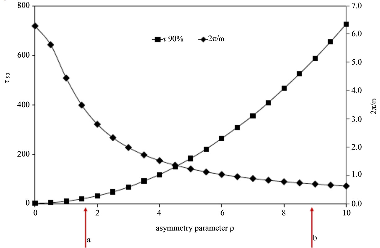
Figure 7. Dependence of  on the asymmetry parameter (squares—left vertical axis) in comparison to the traditional measure of quantum lifetime
  (diamonds—right vertical axis). Atomic units are used. Arrow a marks the asymmetry parameter of 9-hydroxyphenalen-1-one and b marks the parameter for α-methyl-β-hydroxyacrolein. For comparison, the asymmetry parameter for 2-methylnaphthazarin is 9.3 × 10⁵.
to achieve a set probabilistic confidence level (e.g. 90%, 99.999%) that the particle has reached the second state. Unlike approaches based on the (flawed) assumption that the probability that a given orbital is occupied at time  is independent of the probability that the same orbital is occupied at an earlier time t-Δt, the approach yields an answer that converges with decreasing sampling timestep. Application of the method to asymmetric proton transfer yields results that are both consistent with known experimental evidence of tautomerism and more physiccally relevant than the traditional
  measure of life-time. The method of calculation developed here gives a new time-dependent way to analyze and quantify the transport of quantum particles.
7. Acknowledgements
KS thanks C. Rosenthal for numerous valuable discussions as well as and K. Shuford, M. Wander, L. S. Penn and Y. Chen for critical reading of the manuscript. This work was supported by the National Science Foundation grant CHE0449595, including a ROA supplement to support Prof. Kim.
REFERENCES
- R. Baer and D. Neuhauser, Chemical Physics, Vol. 281, 2002, pp. 353-362. doi:10.1016/S0301-0104(02)00570-0
- A. B. Pacheco and S. S. Iyengar, Journal of Chemical Physics, Vol. 133, 2010, Article ID: 044105. doi:10.1063/1.3463798
- H. Guo, L. Liu and K.-Q. Lao, Chemical Physics Letters, Vol. 218, 1994, pp. 212-220. doi:10.1016/0009-2614(93)E1473-T
- C. Joachim, Proceedings of the National Academy of Sciences, Vol. 102, 2005, pp. 8801-8808. doi:10.1073/pnas.0500075102
- A. Nitzan, J. Jortner, J. Wilkie, A. L. Burin and M. A. Ratner, The Journal of Physical Chemistry B, Vol. 104 2000, pp. 5661-5665. doi:10.1021/jp0007235
- W. R. Cook, R. D. Coalson and D. G. Evans, The Journal of Physical Chemistry B, Vol. 113, 2009, pp. 11437- 11447. doi:10.1021/jp9007976
- J.-P. Launay, Chemical Society Reviews, Vol. 30, 2001, pp. 386-397. doi:10.1039/b101377g
- J. A. Hauge and E. H. Støvneng, Reviews of Modern Physics, Vol. 61, 1989, pp. 917-936. doi:10.1103/RevModPhys.61.917
- H. G. Winful, Physics Reports, Vol. 436, 2006, pp. 1-69. doi:10.1016/j.physrep.2006.09.002
- Y. Aharonov, N. Erez and B. Reznik, Physical Review A, Vol. 65, 2002, Article ID: 052124. doi:10.1103/PhysRevA.65.052124
- J. M. Deutch and F. E. Low, Annals of Physics, Vol. 228, 1993, pp. 184-202. doi:10.1006/aphy.1993.1092
- F. E. Low and P. F. Mende, Annals of Physics, Vol. 210, 1991, pp. 380-387. doi:10.1016/0003-4916(91)90047-C
- R. S. Dumont and T. L. Marchioro II, Physical Review A, Vol. 47, 1993, pp. 85-97. doi:10.1103/PhysRevA.47.85
- L. M. Baskin and D. G. Sokolovskii, Russian Physics Journal, Vol. 30, 1987, pp. 204-206.
- P. Pfeifer, Physical Review Letters, Vol. 70, 1993, pp. 3365-3368. doi:10.1103/PhysRevLett.70.3365
- R. J. Gordon and S. A. Rice, Annual Review of Physical Chemistry, Vol. 48, 1997, pp. 601-641. doi:10.1146/annurev.physchem.48.1.601
- D. Bohm, “Quantum Theory,” Prentice Hall, Englewood Cliffs, 1951.
- Mathworks, MATLAB, 1984-2010.
- H. F. Hameka and J. R. de la Vega, Journal of the American Chemical Society, Vol. 106, 1984, pp. 7703-7705 doi:10.1021/ja00337a009
NOTES
*Corresponding author.