Journal of Modern Physics
Vol.3 No.8(2012), Article ID:21674,8 pages DOI:10.4236/jmp.2012.38093
Hidden Mass Boson
Central Institute of Aviation Motors, Moscow, Russia
Email: ivanov@ciam.ru, mamaev@ciam.ru
Received April 29, 2012; revised May 20, 2012; accepted June 11, 2012
Keywords: Vacuum Mathematical Physics; Hidden Mass Boson; Electromagnetic Equations; Conservation Laws; Vacuum Polarization; Displacement Currents; Cosmic Jets; Air Breathing Engines
ABSTRACT
The evidences of the hidden mass boson existence are presented following the fruitful ideas of M. Planck and A. Einstein and using empirical data of modern physics. Within this article main parameters of this mass particle are predicted and its possible structure is analyzed. Moreover, the close system of nonlinear conservative equations and the spread system of Maxwell linear equations are written in the frame of phenomenological description of the hidden mass continuous medium. The displacement current, the Umov-Pointing vector and the physical vacuum polarization have been described adequately in our paper. We discuss some applications of our methodology for simulations of nature and technical device processes. In particular, numerical solutions for cosmic jets and air breathing engines are shown.
1. Introduction
Corresponding to experimental data the density distribution of equilibrium electromagnetic radiation in all frequency range was found by empirical way in 1900 by M. Planck (see, for example, [1]), and is usually written as
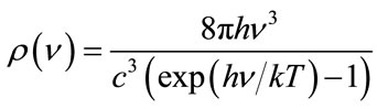
It is used c = 2.998 × 10⁸ m/s—the vacuum light speed, h = 6.626 × 10⁻³⁴ J∙s—the Planck’s constant, k = 1.38 × 10⁻²³ kg(m/s)2/K—the Boltzmann’s constant, T—the absolute temperature. To confirm his formula Planck made the hypothesis that the energy of microscopic objects may accepted only the discrete value, which is proportional by minimal energy hν of virtual resonators.
In connection with this famous formula A. Einstein in 1913 year wrote [2]: “Until now this formula is exactly confirmed by an empirical data, which give numerical values h and k. The great triumph of this paper consists in following. The constant k is taken from the known Boltzmann’s principle, where it is determined by relation

Taken from radiation measurement value k gives, therefore, N, e.g. perfectly accurate the absolute molecule value: to be found, that such way determination of a molecule value is in good correlation with results, getting from the gas theory. Till now there are known another ways for exact determination of N, that brightness confirm the Planck results.”
The fruitful Planck and Einstein ideas, applied to a few last decades of experimental data, light up the future ways of theoretical physics development. Together with L. Boltzmann’s ideas [3] and knowing his constant k they come to the necessity of Hidden Mass Boson (HMB). Even the absence of positive experimental results for the Higgs boson search [4] on the Large Hadrons Collider [5] cannot be a fatal complication for the Standard Model of physics. The responsibility for the baryonic matter birth may consider itself the HMB.
2. Background Radiation Temperature
One of the important achievements of experimental astrophysics of the second half of the XX century was the discovery of the Cosmic Microwave Background (CMB) radiation. The existence of this radiation was predicted by George Gamov in 1948. According to his idea of the origin of the Universe as a result of the Big Bang, the current radiation appeared at the initial stages of the development of the Universe and it was “severed” from the matter spreading this radiation and so far it has cooled off to a very low temperature. The temperature of CMB was predicted by Gamov also (accurate within 7 K). In 1955 the post graduate radio astronomer T.A. Shmaonov in the Pulkovo Observatory experimentally observed noise microwave radiation with the absolute value of the effective temperature 4 ± 3 K. After Shmaonov had defended his dissertation, he also published the article [6].
In 1966 CMB was registered by the American astronomers A. Penzias and R. Wilson [7]. The careful researches of the last decades showed that the distribution of the radiated density does not depend on the direction of its registrations, and that it corresponds to the equilibrium radiation of a black body with the T0 = 2.725 K. These properties of radiation discuss the possibility that we don’t have the case with transformed radiation of stellar objects but with the independent substation filling the entire Universe. According to Ja. B. Zeldovich [8] CMB was sometimes called “new ether”. This name was given as a result of dipole anisotropy discovery of CMB at the middle of 70-year [9]. This circumstance allows the introduction of the absolute cosmological frame of reference in the vicinity of our own Galaxy where the background radiation is isotropic (accurate within smallscale fluctuations).
Before the discovery of CMB with the final value of the temperature T0 it was thought that the temperature in the vacuum of cosmic space is T = 0 K and the pressure of the vacuum is p = 0. These values conformed to the properties of carries of electromagnetic radiations—photons with their rest mass m = 0, the velocity of their moving in a free space can be equal to the speed of light in vacuum c = 2.998 × 10⁸ m/s only, their impulse P and energy E that connect with each other by the formula E = Pc. The photons do not cooperate with each other, and their totality behaves as ideal gas (with the adiabatic index κ = 4/3).
However, the discovery of the final temperature of CMB T0 = 2.725 K should cardinally change the situation. By virtue of the kinetic theory by L. Boltzmann [3] and the dimensional analysis (the π—theorem by E. Buckingham [10]) we come to the final values of pressure p0 and the mass particle m0 in the physics space vacuum [11-14]:

where n—concentration of particles in examining space. Thereby we necessarily introduce with necessarily the ideal gas mass medium to the cosmic space (physical vacuum). This medium can be identified with the mass photon gas or the Dark Matter (DM) of the 20th century or it can also be considered as the classic ether of the 19th century. In the present work for such a medium, the particle structure is based and called Hidden Mass Boson (HMB).
3. Parameters and Structure of HMB
We determine “perfectly accurate the absolute molecule value” at the given temperature of a gas medium and at the speed of light in vacuum c. Write the dimensionless parameter by E. Buckingham [10] , leading to the state equation of ideal gas
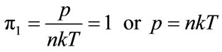 (1)
(1)
If the finite (no zero) values of the concentration n and the temperature T are known, we can calculate gas pressure value p.
Now we write the second dimensionless parameter  that connects pressure, density and characteristic speed of a gas medium
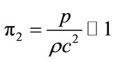 (2)
(2)
and the third parameter  that helps us to estate the mass of the particle (“molecule”) (ρ = nm)
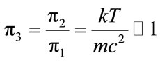 (3)
(3)
So, if taken into account the temperature of gas ideal medium T = 2.725 K, the characteristic light speed c = 2.998 × 10⁸ m/s and the adiabatic constant к = 4/3, we have the exact value of m0 instead of its approach value that formula (3) represents:
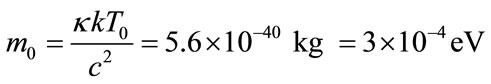 (4)
(4)
This calculated value m0 is the mass of HMB—particle of cosmic space.
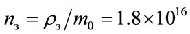
Now we calculate the parameters of this medium for two cases: for the whole Universe, knowing the approximation values its critical density  kg/m3 and near the Earth if
  ~10–23 kg/m3. Using the formula (2) we reach the estimation for the critical pressure of the Universe
And the value of pressure  nears the Earth
 (5)
(5)
The concentrations have the following values
 (6)
(6)
and
 (7)
(7)
Thus, we have come to know the method that was suggested by A. Einstein. In this method “the value k was received by measuring radiation and gives, therefore, N, i.e. perfectly accurate the absolute molecule value” with mass .
.
In this respect, we must make two very important remarks. First, in such approach the virtual emitted Plank resonators have been replaced by real HMB particles. The problem of the radiation transfer will be examined in the next part of our paper. Using fourth dimensionless parameter
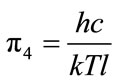
we may determine the mean free path length l of the HMB in a free space, if the temperature is T0 = 2.725 K
 (8)
(8)
For the free space volume  of the Universe from (6) we have the number of the HMB particles that is roughly 2.7 × 10⁶.
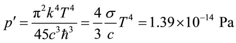
The second remark concerns to the appreciation of value  that was measured with the formula (5) and confirmed by experiment. Calculation of the photon gas radiation pressure
 , as a given the temperature T0 can be carried out by traditional way (see, for example, [15- 17]), using the formula
This value of the perturbed pressure (in far field  ~
~ ) is distinguished from its pressure (see [14]) by the multiplier c. So we have
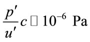 (9)
(9)
that corresponds to appreciation (5). In this example we can see analogy with the sound perturbed gas pressure in the far field and the full gas pressure in the source [18]. The sound pressure far from the source of noise is on principle distinguished from the pressure directly inside of the source (this difference is characterized by multiplier which contain the value of the speed of disturbance propagation in this case for sound speed of light c).
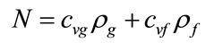
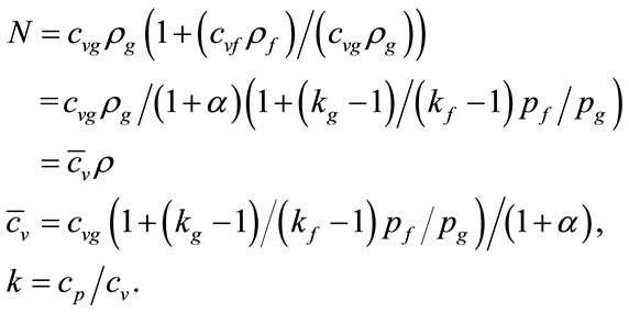
It is easy to calculate the gas constant R and the specific heats  and
and  for the HMB medium [14]
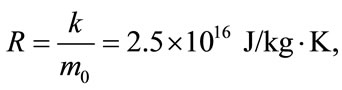
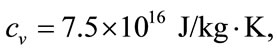
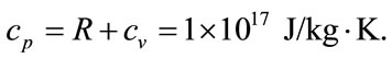
We also have the traditional state equation of gas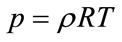 .
.
Now we examine the problem of the definition for more real the HMB structure. The demand of modeling is particularly important for vacuum polarization [19], for the displacement current by Maxwell [20], entering to electrodynamics equations, and for the Umov-Pointing vector of electromagnetic energy flux.
According to [12,13], we take the HMB structure as a classical dipole. Proceeding from the appreciations of mass and charge for proton and electron we obtain the liner size of the dipole 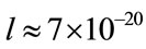 m and its charge
 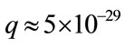 C. The value of the electric dipole moment p = q·l ≈ 3.5 × 10–48 C·m. In spite of its miniature size we consider that all known properties of electric dipoles are retained. Thus we’ll carry out the above mention properties for the vacuum polarization. We write the equation for gas that submits to the Fermi statistics and to the Bose statistics. In this case the dimensionless parameter
  has form [14,15]
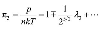
where the signs  correspond to Bose & Fermi gases and
 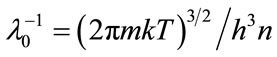 is the statistical sum for one particle. The second term as well as the higher terms in the right side of this formula come from quantum mechanics. The value in series is valid for
  or for
 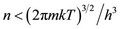 . The expression
  is the length of de Broil wave and
  is a quantity of heat energy
  of particle. Thus, the Bose statistics can be employed for the HMB gas, that we introduced using the dimensional analysis and thermodynamics. The problem of the condensed state of the HMB gas has issues with low temperature and high pressure that can be of interest if it is further examined.
In the offering model of physical vacuum the electronpositron pair birth [21] is simulated by natural way. A creation of this pair came from material medium and not from the emptiness with all conservation law observance: mass, charge, impulse and energy. In our case, a creating of the pair can be interpreted as destruction of a sufficiently large number of dipoles under strong enough electric field.
At the end of this part, we want to show the experimental evidence for the existence of the HMB gas medium. According to the current analysis the propagation velocity of perturbation in vacuum has to depend on the temperature (in particular, from (3) we have c ~ sqrt(T)). Therefore, the speed of light in vacuum с = 2.998 × 10⁸ m/s has not been limited. The experiments of [22] clearly demonstrate this fact and allow giving additional experimental confirmation of the conclusions of our research.
4. Modified Maxwell Equations of Electrodynamics in Free Space
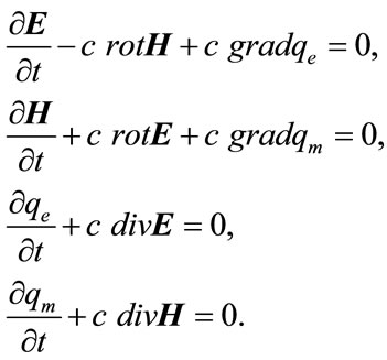
In the medium of physical vacuum being examined the longitudinal and transverse waves will propagate in the electromagnetic field. The system of linear equations, describing the propagation of electromagnetic disturbances can be written in the form [13,22,23]
 (10)
(10)
with the purpose of longitudinal waves modeling into tradition system of electrodynamics equations of a free space, the scalar field  and
and  were introduced and that represents the density of force lines of electric and magnetic field. The first term in the first equation of the system (10) is a time change of E and the displacement current in vacuum.
The system of Equation (10) describes the propagation of all parameters of disturbances with the same speed c. It is easy to prove, differentiating the first two equations with respect to t:

that, by using the formula of vector analysis
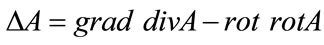
leads to the wave equations for the changes E and H
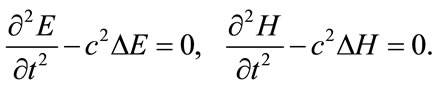
The changes of scalar field qe and qm, as well as scalar and vector potentials of E and H can be also lead to the wave equations.
The system of linear Equations (10) describes the propagation with equal velocities both the longitudinal waves (the wave of compression and rarefaction) and the transverse wave (share wave) in a homogeneous isotropic space. At the same time, the modeling of longitudinal wave is provided by the introduction additionally of the scalar fields qe and qm to the system Maxwell equations. In this connection, we can call the scalar fields qe and qm as fields of density (force lines), connecting with fields E and H. In principle, it is not difficult to examine the case when propagation velocities of longitudinal and transverse waves in the electromagnetic field are different.
5. Displacement Current, Electromagnetic Energy Flux, Current in a Conductor and Self Inductance
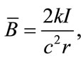
The proposed physical model of vacuum and the suggested structure of the HMB give very clear interpretation of the Maxwell displacement current and the UmovPoynting vector [24]. Firstly, we are reminded of the spread example of necessity to introduce the displacement current to the Ampere’s law. For instance, a parallel plate capacitor with circular plates is charged by current I (see Figure 1). The magnetic field in the point P at a distance r from the conductor can be calculated by Ampere’ law
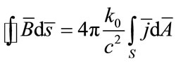
Integrating with respect to the circle we will obtain the magnetic field in the point P
where  is summed current flowing through the surface S. The Ampere’s law has to issue for surface S¢, that is based on the same circle but coming between plates of the capacitor. By adopting this method the availability of current and electric field between the plates of the capacitor, the displacement current is introduced and the Ampere’s law has an additional term
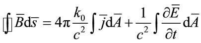
The last term was introduced by Maxwell (and was named the displacement current). The physical meaning of the displacement current in our case is the displacement of dipoles of HMB and their re-orientation between the plates of the capacitor. In vacuum (when dielectric is absent) availability of the displacement current between the plates of the capacitor comes to the polarization of real HMB dipoles and we see clean and real physical interpretation of this current.
Now we examine the Umov-Poyting vector U of the electromagnetic energy flux. With changing of electric field E within capacitor, its internal volume acquires energy U with velocity

The energy flux is described by the Umov-Poynting vector  and has direction from the edges of the plates to inside of the capacitor (Figure 1) from its surrounding space. As well as the displacement current in our case (availability of the HMB dipoles) the energy flux of electric field has physical meaning and connects with the moving (flowing) of dipoles from surrounding to inside.
The propagation of current inside the conductor takes place when the incidence of electric potential along the conductor and the availability drops electric field  inside and close to the conductor which in turn is directed
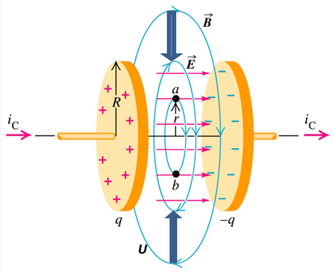
Figure 1. Displacement current the Umov-Poyting vector.
alongside the conductor. Availability of the current induced magnetic field  around the conductor is directed on tangent to the circle around the wire. The vectors
  and
and  are perpendicular. There is energy that flows to the inside of the conductor from all sides and which accompanies energy lost by the conductor as heat.
The classic theory shows that electrons take their energy from outside, which means from the energy flux of the outside field to the inside of the conductor. Existed HMBs in electric dipole form are created by the energy flux going to the conductor, which in turn is processing electric current along it more clearly.
The same natural interpretations we get to known phenomena of inductance and self inductance.
6. The Conservation Laws for Two Components Electrically Neutral Medium
From the view point of practical applications further examining of problems of the moving of radiating medium will be done within the two-component model of radiating gas [14,25]: classic gas and radiation (gaseous HMB medium) components.
Here is the full system of equations, describing the conservation laws for this model. We will write all parameters being used in the usual way and with index: ggas, f-radiation components (for example, we write density as ρg and ρf). However, we will write without index the total value of density, pressure and energy.
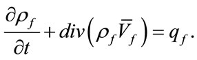
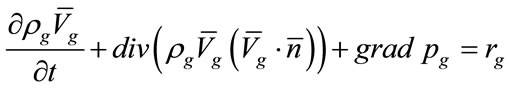
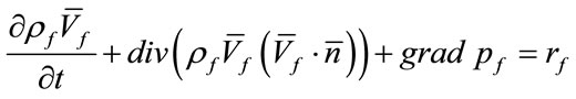
The conservation laws for mass, and energy, written in divergent form for every component are
 (11)
(11)
 (12)
(12)
 (13)
(13)
 (14)
(14)
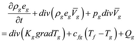 (15)
(15)
 (16)
(16)
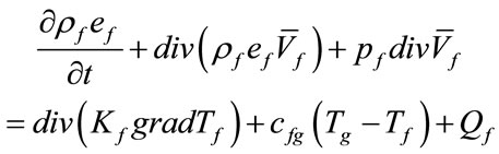
The system of Equations (11)-(16) refers to heat conductive gas and radiated components (the first terms in the second side of equation Kg and Kf are coefficient of temperature-conductive for gas and radiation components respectively. The second terms in the second side of the Equations (16) and (17) characterize the energy exchange between gas and radiation components. The last terms Qg and Qf are an extra source of energy (stocks), that take into account the presence of extra channels of energy exchange (for example in the case of chemical transformations). The system of Equations (11)-(16) are closed by equations for the state of gas and radiation components.
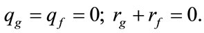
Undoubtedly, the general solution of this system involves considerable difficulties even in the final formulation of the problem, since the values for change in coefficients have to be defined more precisely. It will be much easier if we consider as zero approximation the case of single speed motion of the phases, and if thermodynamic equilibrium between them is available:
 (17)
(17)
We also take into consideration that external sources of mass, momentum and mass change between component are absent in the examining area of flow
Then, following [18], write the mass continuity equations of each phase in form:
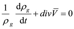
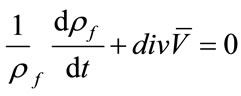
or

The last equality talks about conservation of quantity
 (18)
(18)
along the stream lines and if it is proposed that at the initial time the ratio of the densities is constant but does not depend on the coordinate, then Equation (18) will be correct in any point of flow.
Now we have found the total conservation laws for both component of medium.
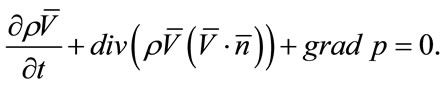
Adding (11) to (12) and (13) to (14) and taking into consideration the assumptions that have been made, the equations of continuity and motion of the one component medium have the next form:

The total equation of energy has little change. Adding (15) to (16) we will obtain:
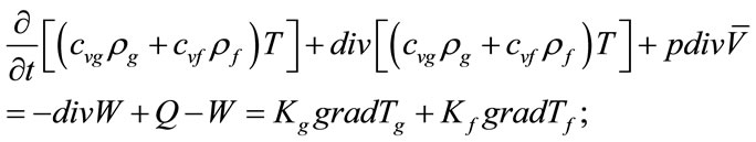
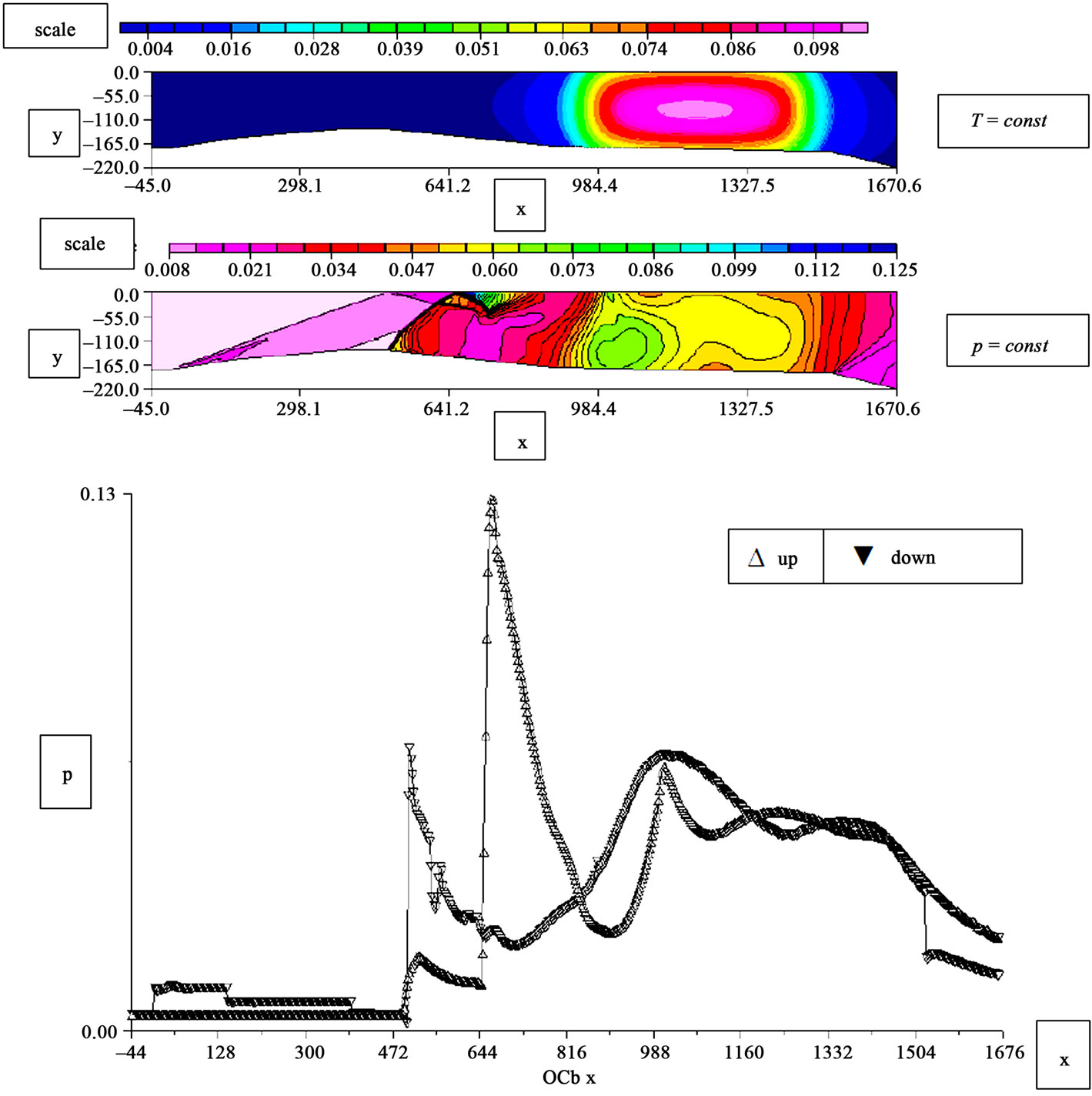
Figure 2. Pressure distributions in channel with intensive heat addition and radiation effects.
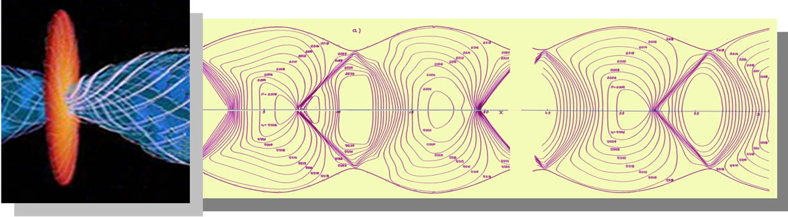
Figure 3. Cosmic jet simulation.
In order to give the equation of energy the usual form, we will be required to undertake the following:
by the next step:
You will recall, that according to (18),  is constantly along the stream lines. Therefore, if Tf=Tg then the ratio
  is constant as well. We do the same with the state equation for total component of the system:

The equation of energy with –div S in the right hand side, where the flow of radiation S = sT4, often used for modeling of radiation gas flows.
For further analysis, using this approximation, obtain the next system of equations describing single speed equilibrium flow of radiated gas with mass radiating component:
 (19)
(19)
Obviously, if rf = 0 we have the usual system of gas dynamics for one component radiated medium.
7. Examples of Numerical Solutions
The efficiency of the equations system that was given in the previous part can be shown by using two examples:
1) in model channel of high-speed air jet engine with intensive heat application;
2) in a space jet, expiring from the center of quasars and active galactic.
First, we present the examples of breaking the stream of the incoming flow with the number of Mach М0 = 4 in the plane channel similar to the channel of [26] by its form. The integration of the system (19) with the extra term in the right-hand side imitating the supply of heat was carried out according to the Godunov scheme [27] with a second order of accuracy. In the upper part of Figure 2 can be seen the channel scheme, place and intensity of high-energy fuel supply. The channel consists of air-intake of mixed compression, part of combustion chamber and expanding nozzle. In Figure 2 the flow is shown as constant pressure lines and distributions of statistic pressure along upper and lower walls of the model. We can see a complicated system of shocks taking place that occur in the cross-section of the throat in the channel. In the combustion chamber there is a pressure increase in the initial part of supply of the flue area and the flow chocking in the vicinity of the nozzle entry.
In the second example of accounting for superluminal space ax symmetric flow, expiring from the center of quasar, the system (19) when the parameter (18) , was integrated according to stationary analogy of Godunov method [27]. In Figure 3 can be seen a few first “barrels” of under expanded jet with a stationary structure of stream in them with the lines of constant pressure.
Concluding this article we wish to emphasize again that the ideas of Planck, Einstein and Boltzmann of taking the temperature of physical vacuum T = 2.725 K lead to the final outcome of the necessity for HMB existence, which in turn can be the receiver of elusive Higgs boson.
The authors express their gratitude to B. O. Muravjov for his help.
REFERENCES
- M. Planck, “Theorie der Warmestrahlung,” 1927.
- A. Einstein, “Max Planck as Researcher,” Nauka, Moscow, 1967.
- L. Boltzmann, “Lectures on Gas Kinetic Theory,” GITTL, Moscow, 1956.
- P. W. Higgs, “Broken Symmetries, Massless Particles and Gauge Fields,” Physics Letters, Vol. 12, No. 15, 1964, pp. 132-133. doi:10.1016/0031-9163(64)91136-9
- The LHC Experiments. GERN, 2011.
- Т. А. Shmaonov, “Methodology of Absolute Measurements for Effective Radiation Temperature with Lower Equivalent Temperature,” Apparatuses and Technics of Experiment, No. 1, 1957, pp. 83-86.
- A. A. Penzias and R. W. Wilson, “A Measurement of Excess Antenna temperature at 4080 m/s,” The Astrophysical Journal, Vol. 142, 1965, pp. 419-421. doi:10.1086/148307
- A. D. Dolgov, Ja. B. Zeldovich and M. V. Sagin, “Cosmology of Earlier Universe,” MSU, Moscow, 1988.
- G. F. Smooth, “Anisotropy of Background Radiation,” Uspekhi Fizicheskih Nauk, Vol. 177, No. 12, 2007, pp. 1294-1318.
- E. Buckingham, “On Physically Similar Systems; Illustrations of the Use of Dimensional Equations,” Physics Review, Vol. 4, No. 4, 1914, pp. 345-376. doi:10.1103/PhysRev.4.345
- L. I. Sedov, “Methods of Similarity and Dimension in Mechanics,” Nauka, Moscow, 1967.
- M. Ja. Ivanov, “To Analogy of Gas Dynamics and Electrodynamics Models,” Fizicheskaya Misl Rossii, No. 1, 1998, pр. 1-14.
- M. Ja. Ivanov, “Dynamics of Vector Fields in a Free Space,” Mathematics Modeling, Vol. 10, No. 7, 1998, pp. 3-20.
- M. Ja. Ivanov, “Thermodynamically Compatible Conservation Laws in the Model of Heat Conducting Radiating Gas,” Computational Mathematics and Mathematical Physics, Vol. 51, No. 1, 2011, pp. 133-142. doi:10.1134/S096554251101009X
- A. Isihara, “Statistical Physics,” Academy Press, Seattle, 1973.
- А. I. Anselm, “Bases of Statistical Physics and Thermodynamics,” Nauka, Мoscow, 1973.
- J. B. Zeldovich and Y. P. Riezer, “Physics of Shock Waves and High Temperature Gas Dynamics Phenomena,” Nauka, Мoscow, 1966.
- L. G. Loytcansky, “Mechanics of Fluid and Gas,” Nauka, Мoscow, 1973.
- L. B. Оkun, “Physics of Elementary Particles,” Editorial, Мoscow, 2005.
- J. K. Maxwell, “Selected Papers on Electromagnetic Field Theory,” GTTL, Мoscow, 1952.
- D. L. Burke, et al., “Positron Production in Multiphoton Light-by-Light Scattering,” Physics Review Leters, Vol. 79, No. 1, 1997, pp. 1626-1629. doi:10.1103/PhysRevLett.79.1626
- Ju. I. Malakhov, M. Ja. Ivanov, N. Q. Shi and V. V. Schaulov, “Registration of Temperature Dependence for Electromagnetic Front Velocity with Theoretical Support and Demonstration Examples,” 2012.
- M. Ja. Ivanov and L. V. Terentieva, “Gasdynamic Elements of Dispersive Medium,” Informconversion, Moscow, 2004.
- R. Feiman, R. Leiton and M. Sands, “Lectures on Physics,” 1964.
- M. Ja. Ivanov, “Dark Matter—Quo Vadis?” ICATPP Conferences, Como, 3-7 October 2011, p. 68.
- V. L. Semenov, A. N. Prochorov, M. V. Strokin, V. L. Relin and V. Y. Alexandrov, “Fire Tests of Experimental Scramjet in Free Stream in Continuously Working Test Facility,” AIAA Paper No. 2002-5211.
- S. K. Godunov, A. V. Zabrodin, M. Ja. Ivanov, A. N. Kraiko and G. P. Prokopov, “Numerical Solution of Multidimensional Gas Dynamics Problems,” Nauka, Moscow, 1976.